8.2. Sampling Variability

Goals

• Explain sampling variability and why repeated samples differ

• Visualize sampling distributions with simulation

• Connect standard error to sample size

• Recognize law of large numbers behavior

import numpy as np
import pandas as pd
import seaborn as sns
import matplotlib.pyplot as plt

sns.set_theme()

We will simulate many samples from a Bernoulli process (think weighted coin with \(p=0.6\) for heads) to see how sample proportions vary.

Key quantities:

• True proportion \(p\)

• Sample size \(n\)

• Sample proportion \(\hat p\)

• Sampling distribution: distribution of \(\hat p\) across repeated samples

8.2.1. Simulating Sample Proportions

rng = np.random.default_rng(seed=0)

p_true = 0.6
n = 40
n_sims = 5_000

# Draw many samples and compute sample proportions
samples = rng.binomial(n=n, p=p_true, size=n_sims)      # Draw samples from a binomial distribution
sample_props = samples / n                              # Compute sample proportions    

summary = pd.Series(sample_props).describe(percentiles=[0.025, 0.5, 0.975]).round(3)
summary

count    5000.000
mean        0.600
std         0.078
min         0.350
2.5%        0.450
50%         0.600
97.5%       0.750
max         0.850
dtype: float64

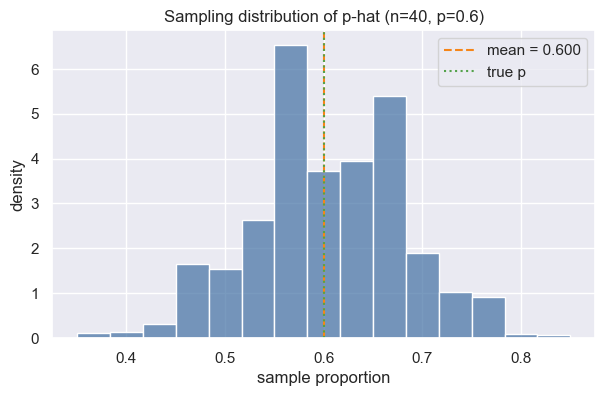
We see that

• 97.5% of the simulated sample proportions fell at or below 0.750.

• 2.5%, the lower bound, is 0.450.

• the middle 95% of simulated proportions fall between 0.45 and 0.75.

Now let us take a look at the sample distribution: he distribution of sample proportions (sample_props) generated from 5,000 simulated samples.

8.2.2. Sampling Distribution

fig, ax = plt.subplots(figsize=(7, 4))
sns.histplot(sample_props, bins=15, stat="density", color="#4c78a8", edgecolor="white", ax=ax)

ax.axvline(sample_props.mean(), color="#f58518", linestyle="--", label=f"mean = {sample_props.mean():.3f}")
ax.axvline(p_true, color="#54a24b", linestyle=":", label="true p")
ax.set(xlabel="sample proportion", ylabel="density", title="Sampling distribution of p-hat (n=40, p=0.6)")
ax.legend()
plt.show()

8.2.3. Standard Error

For a sample proportion, the standard error measures the typical deviation of \(\hat p\) from \(p\):

\(\text{SE}(\hat p) = \sqrt{\dfrac{p(1-p)}{n}}\)

If \(p\) is unknown, we often plug in \(\hat p\). In real data analysis you don’t know p, so you’d substitute it with p-hat instead. It’s an approximation, but a good one for large n.

\(SE\) is what “sampling variability” is, expressed as a single number. p-hat is the sample proportion, e.g., 0.6.

The standard deviation of the sampling distribution (simulation/empirical) of p-hat is the standard error by definition.

Note that:

• p(1−p) is the variance of a single observation. It captures how much “spread” there is in one yes/no trial.

  • p(1−p) is maximized at p=0.5 (most uncertain) and shrinks as p approaches 0 or 1.

  • e.g. if p=0.6 → 0.6×0.4 = 0.24

• “plug in p̂”: In real life you don’t know p (that’s why you’re sampling!), so you substitute your observed p̂ into the formula. It’s an approximation, but it works well for reasonably large n.

Here we compare the empirical SD of simulations vs. the theoretical SE, to confirm that they match. In the comparison below, ddof stands for Delta Degrees of Freedom. It controls the denominator used in the std calculation. If ddof=0, divides by n (population std); if ddof=1, divides by n−1 (sample std).

• The theoretical SE is the formula applied to the known values:

  sqrt(0.6 × (1-0.6) / 40) ≈ 0.0775.
  

• The empirical SE is the standard deviation of the 5,000 simulated p-hat values – no formula, purely from the simulation.

• If the theoretical SE comes out nearly identical with the empirical (simulation) SE, the it validates that the formula is correct and the simulation is working as expected.

se_theoretical = np.sqrt(p_true * (1 - p_true) / n)
se_empirical = sample_props.std(ddof=1)

print(f"Theoretical SE: {se_theoretical:.4f}")
print(f"Simulated SE:   {se_empirical:.4f}")

Theoretical SE: 0.0775
Simulated SE:   0.0781

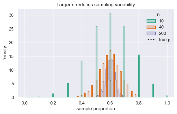
8.2.4. Effect of Sample Size

Larger samples shrink variability. Below we compare sampling distributions (p-hats) across different \(n\) while keeping \(p=0.6\) fixed.

def simulate_props(n, p=0.6, sims=5_000):
    props = rng.binomial(n=n, p=p, size=sims) / n   # Simulate sample proportions by drawing from a binomial distribution and dividing by n
    return props

ns = [10, 40, 200]
records = []
frames = []
for n_i in ns:
    props_i = simulate_props(n=n_i)
    frames.append(pd.DataFrame({"n": n_i, "prop": props_i}))    # Store the sample proportions in a DataFrame for plotting
    records.append({
        "n": n_i,
        "mean(p-hat)": props_i.mean(),
        "sd(p-hat)": props_i.std(ddof=1),
        "SE formula": np.sqrt(p_true * (1 - p_true) / n_i)
    })

display(pd.DataFrame(records).round(4))

plot_df = pd.concat(frames, ignore_index=True)
fig, ax = plt.subplots(figsize=(7, 4))
sns.histplot(data=plot_df, x="prop", hue="n", element="step", stat="density", common_norm=False, palette="Dark2", ax=ax)
vline = ax.axvline(p_true, color="black", linestyle=":")
ax.set(xlabel="sample proportion", title="Larger n reduces sampling variability")

leg = ax.get_legend()
handles = list(leg.legend_handles) + [vline]
labels = [t.get_text() for t in leg.get_texts()] + ["true p"]
ax.legend(handles=handles, labels=labels, title="n")
plt.show()

	n	mean(p-hat)	sd(p-hat)	SE formula
0	10	0.5994	0.1549	0.1549
1	40	0.5984	0.0780	0.0775
2	200	0.5986	0.0348	0.0346

Takeaways

• Repeated samples vary; summarizing their distribution clarifies how much.

• Standard error captures typical sampling fluctuation and shrinks as \(n\) grows.

• Simulations help check formulas and build intuition about variability.

As 𝑛 gets larger, the 𝑝-hat values from repeated samples cluster more tightly around the true 𝑝. In the plot, the histogram for 𝑛 = 200 is much narrower than for 𝑛 = 10 — the same true 𝑝 = 0.6, but larger samples give you estimates that are consistently closer to it.

Concretely, the SE formula shows why: SE = sqrt(𝑝(1−𝑝)/𝑛), so as 𝑛 increases, SE decreases. A larger sample gives you more information, so your estimate is less noisy.