3. NumPy Arrays

Click on the figure to enlarge it for clearer view

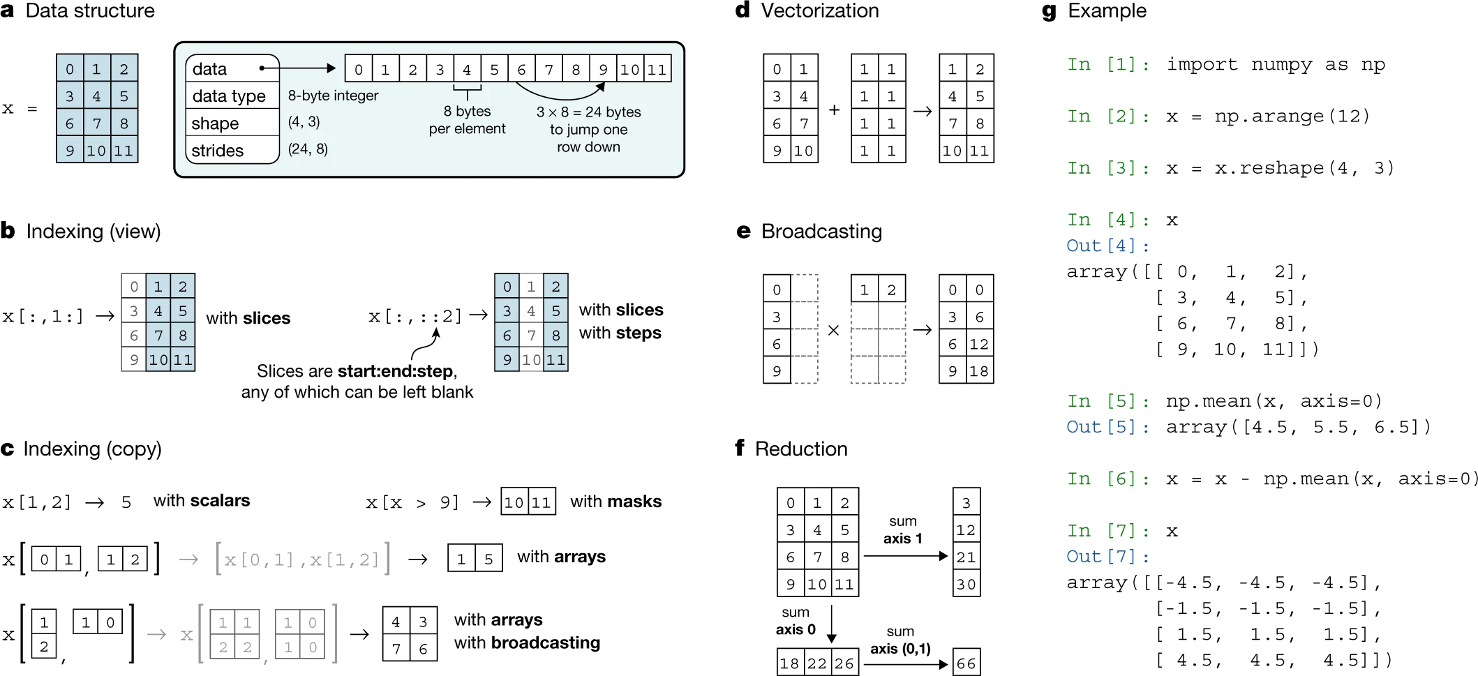
Fig. 3.1 Numpy Array Concepts

NumPy organizes array operations along axes, masks, and broadcasting rules. Fig. 3.1 above summarizes how these concepts interact when reducing or slicing arrays [Harris et al., 2020].

NumPy, short for Numerical Python, is the foundation for Python’s data science ecosystem. Nearly all Python libraries for data science, machine learning, and scientific computing—including pandas, scikit-learn, and TensorFlow—build on NumPy. Understanding NumPy means understanding how these tools work under the hood.

NumPy’s core strength is its ndarray (N-dimensional array), which provides fast, memory-efficient operations on large datasets through built-in tools for math, statistics, and linear algebra.

What You'll Learn

This chapter covers NumPy fundamentals with emphasis on practical array operations:

1. NumPy Basics

   • Creating arrays

   • Array attributes (shape, dtype, ndim)

   • Indexing and slicing

   • Reshaping and concatenation

2. Universal Functions (ufuncs)

   • Vectorized operations

   • Element-wise arithmetic

   • Comparison and Boolean operations

   • Broadcasting rules

3. Random Number Generation

   • Random sampling

   • Statistical distributions

   • Reproducible randomness with seeds

   • Simulation techniques

NumPy provides built-in tools for math, statistics, and linear algebra. NumPy makes numerical computing in Python fast, efficient, and powerful.

As an introduction, we need to learn the following about NumPy with an emphasis on ndarrays:

1. Basics of NumPy arrays

   1. Data Structure

   2. Creating Arrays

   3. NumPy Random Module

   4. Indexing and Selection

   5. Array Attributes

2. NumPy array operations

   1. 2.1. Vectorized Operation

   2. 2.2. Arithmetic ufuncs

   3. Aggregation

   4. Advanced Features:

      1. Aggregations

      2. Broadcasting

      3. Comparison

      4. Fancy indexing

      5. Sorting

3. NumPy Randomness