Arrays Basics

3.1. Arrays Basics#

import matplotlib
import IPython
print(f"matplotlib: {matplotlib.__version__}")
print(f"IPython: {IPython.__version__}")

matplotlib: 3.10.8
IPython: 8.38.0

NumPy arrays (N-dimensional arrays, or ndarray) are a powerful extension of Python lists, offering compact storage and fast operations for numerical data in rows and columns.

While NumPy arrays can have any number of dimensions, the most common are:

Vectors: 1-dimensional arrays with a single axis
Matrices: 2-dimensional arrays with two axes (rows and columns)

This section covers core concepts for working with NumPy arrays:

Array data structure
Creating arrays
Indexing and slicing
Array attributes (ndim, dtype, shape) and functions like reshape()

The primary data structure in NumPy is the N-dimensional array, or ndarray. NumPy’s arrays are a list of lists in Python, but are more compact than Python lists. In essence, a Python list is an array of pointers to heterogeneous Python objects, while a NumPy array is an array of uniform values of the same type (e.g., all integers, all floats) and array elements are stored in one continuous block of memory, similar to how arrays work in C (Fig. 3.2). Python lists are more flexible, but Numpy arrays are smaller in file size, and access in reading and writing items is much faster [Martelli, 2009].

3.1.1. NumPy Environment#

3.1.2. Data Structure#

The primary data structure in NumPy is the N-dimensional array, or ndarray. NumPy’s arrays are a list of lists in Python, but are more compact than Python lists. In essence, a Python list is an array of pointers to heterogeneous Python objects, while a NumPy array is an array of uniform values of the same type (e.g., all integers, all floats) and array elements are stored in one continuous block of memory, similar to how arrays work in C (Fig. 3.2). Python lists are more flexible, but Numpy arrays are smaller in file size, and access in reading and writing items is much faster [Martelli, 2009], which is a huge advantage when dealing with large datasets.

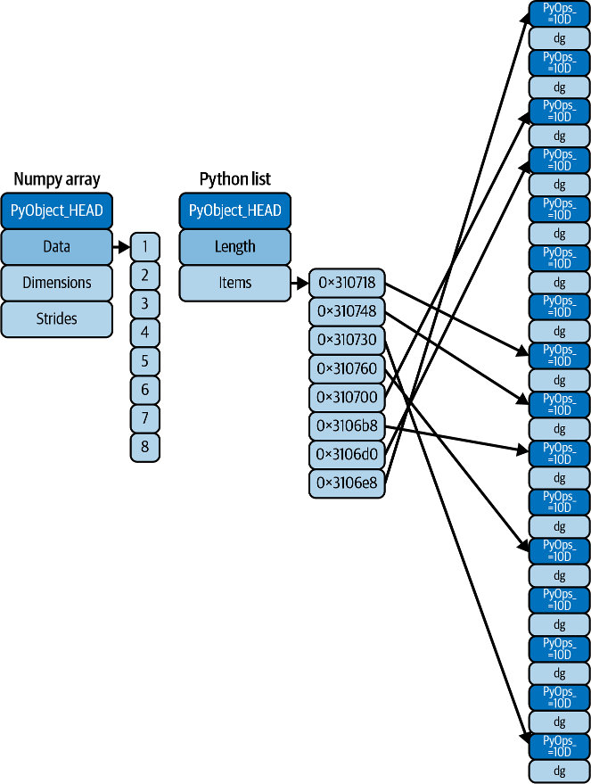
c-vs-python-list — Fig. 3.2 Difference between NumPy array (C) and Python lists [Vanderplas, 2022]#

In short, NumPy’s primary data structure is the ndarray (N-dimensional array), which is a homogeneous, multidimensional array of fixed-size items. This means all elements within a ndarray must be of the same data type (note: To store heterogeneous data, NumPy uses structured arrays). While Python defines only one type of a particular data class (there is only one integer type, one floating-point type, etc.), there are 24 new fundamental Python types to describe different types of scalars in NumPy.

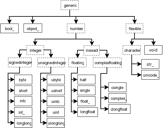
np-array-data-types — Fig. 3.3 Hierarchy of type objects representing the array data types (NumPy: Scalars)#

Compared to Python built-in types:

Python type	NumPy type
`int`	`int_`
`bool`	`bool_`
`float`	`float64`
`complex`	`complex128`
`bytes`	`bytes_`
`str`	`str_`
`memoryview`	`void`
(all others)	`object_`

In NumPy, the terms scalar, vector, and matrix refer to specific dimensions of these arrays.

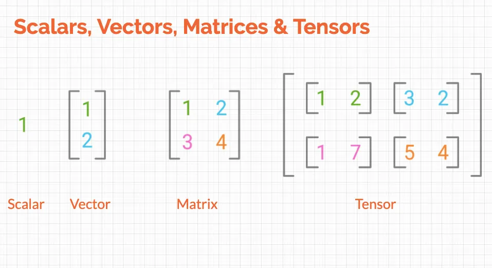
scalar-vector-matrix-tensor — Fig. 3.4 Scalar, Vector, Mmatrix, and Tensor (Harshit Tyagi)#

NumPy is Python’s linear algebra library; therefore, its terminology is commonly used for data science. Some of the essential terms are {cite}``:

Scalar: Any single numerical value is a scalar, as shown in the image above. It is simply denoted by lowercase and italics. For example: n.
Vector: An array of numbers(data) is a vector. You can assume a column in a dataset to be a feature vector.
Matrix: A matrix is a 2-D array of shape (m×n) with m rows and n columns.
Tensor: Generally, an n-dimensional array where n>2 is called a Tensor. But a matrix or a vector is also a valid tensor.

3.1.3. Using NumPy#

3.1.3.1. Installing NumPy#

To install NumPy, you would:

Go to the command line
Navigate to your project directory (dsm)
Activate the virtual environment
Issue the pip install [package] syntax to install:

pip install numpy

You should see the installation happens like:

(.venv) tychen✪macː~/workspace/dsm$ pip install numpy
Collecting numpy
Downloading numpy-2.3.3-cp312-cp312-macosx_14_0_arm64.whl.metadata (62 kB)
━━━━━━━━━━━━━━━━━━━━━━━━━━━━━━━━━━━━━━━━ 62.1/62.1 kB 1.3 MB/s eta 0:00:00
Downloading numpy-2.3.3-cp312-cp312-macosx_14_0_arm64.whl (5.1 MB)
━━━━━━━━━━━━━━━━━━━━━━━━━━━━━━━━━━━━━━━━ 5.1/5.1 MB 4.1 MB/s eta 0:00:00
Installing collected packages: numpy
Successfully installed numpy-2.3.3

Note

Alternatively, in a Jupyter notebook, you may use the %pip install [package] syntax in a code cell to install packages just like pip install [package] in the command line. You will also see people use the older syntax !pip install, which runs pip as a shell command, while %pip is a Jupyter magic function that runs in the current notebook kernel, allowing you to customize your notebooks.

Don’t forget to comment out (#) your pip commands in the cells after installation, or they’ll run every time you run the cell.

3.1.3.2. `import` NumPy#

Once you’ve installed NumPy, you can import it as a library and give it an alias; conventionally we calle it np:

import numpy as np

Here, np is an alias for numpy, and the dot notation gives us access to the contained objects, such as array() in this case.

After you import the library, you use the dot operator to access the methods/functions and attributes inside the module/library. Just type the name of the object, and then the dot (.) and the Tab key to show the menu. You can scroll down to select the methods. In this case, we choose the array method (note: the Tab key can also do autocompletion).

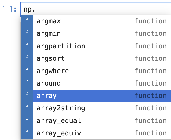
../../_images/dot-operator-numpy.png — Fig. 3.5 Using the dot operator and Tab completion in NumPy#

3.1.3.3. Functions#

Just as Python lists do, NumPy provides many built-in functions and capabilities. For example:

Category	Function	Description	Example
Array Creation	`np.array()`	Create array from list or sequence	`np.array([1, 2, 3])`
	`np.arange()`	Create array with evenly spaced values	`np.arange(0, 10, 2)`
	`np.linspace()`	Create array with specified number of elements	`np.linspace(0, 10, 5)`
	`np.zeros()`	Create array filled with zeros	`np.zeros((3, 4))`
	`np.ones()`	Create array filled with ones	`np.ones((2, 3))`
	`np.eye()`	Create identity matrix	`np.eye(3)`
	`np.full()`	Create array filled with specified value	`np.full((2, 3), 7)`
Reshaping	`np.reshape()`	Change array shape	`arr.reshape(2, 5)`
	`np.flatten()`	Flatten to 1D array	`arr.flatten()`
	`np.transpose()`	Transpose array	`arr.transpose()` or `arr.T`
	`np.concatenate()`	Join arrays together	`np.concatenate([arr1, arr2])`
	`np.stack()`	Stack arrays along new axis	`np.stack([arr1, arr2])`
Indexing/Selection	`np.where()`	Indices where condition is true	`np.where(arr > 5)`
	`np.nonzero()`	Indices of non-zero elements	`np.nonzero(arr)`
	`np.select()`	Select elements based on conditions	`np.select([cond1, cond2], [val1, val2])`
Array Operations	`np.sum()`	Sum of array elements	`np.sum(arr)` or `arr.sum()`
	`np.sort()`	Sort array	`np.sort(arr)`
	`np.argsort()`	Indices that would sort array	`np.argsort(arr)`
	`np.unique()`	Unique elements in array	`np.unique(arr)`
Random	`np.random.rand()`	Random floats in [0, 1)	`np.random.rand(3, 4)`
	`np.random.randn()`	Random values from standard normal distribution	`np.random.randn(5)`
	`np.random.randint()`	Random integers in specified range	`np.random.randint(0, 10, 5)`
	`np.random.choice()`	Random sample from array	`np.random.choice([1, 2, 3], 5)`
	`np.random.shuffle()`	Randomly shuffle array in place	`np.random.shuffle(arr)`
Math	`np.clip()`	Limit values to range	`np.clip(arr, 0, 10)`
	`np.abs()`	Absolute value	`np.abs(arr)`
	`np.round()`	Round to nearest integer	`np.round(arr, 2)`
	`np.mean()`	Mean (average) of array	`np.mean(arr)` or `arr.mean()`
	`np.std()`	Standard deviation	`np.std(arr)` or `arr.std()`
	`np.min()` / `np.max()`	Minimum/maximum value	`np.min(arr)` / `np.max(arr)`

3.1.4. Creating NumPy Arrays#

3.1.4.1. `array([sequence])`#

You can create an array by directly converting a list to an array. Let us create a list first:

num_list = [1,2,3, 4, 5]
print("num_list: ", num_list)
print("num_list type:", type(num_list))

num_list:  [1, 2, 3, 4, 5]
num_list type: <class 'list'>

Now let’s convert the list into a numpy array using numpy’s array() function to create a 1-D array.

arr = np.array(num_list)       ### casting a list to a numpy array
arr

array([1, 2, 3, 4, 5])

Now let’s create a 2-D (rows and columns) array using a 2-D tuple:

arr_2d = np.array(
    (
        [1,2,3],
        [4,5,6],
        [7,8,9]
    )
)
arr_2d

array([[1, 2, 3],
       [4, 5, 6],
       [7, 8, 9]])

An example of Python 3-D list, which is a list of lists:

list_of_list = [
    [
        [1, 2, 3], 
        [2, 2, 3], 
    ], 
    [
        [3, 2, 3],
        [4, 2, 3]
    ],
    [
        [5, 2, 3], 
        [6, 2, 3]
    ]
]
list_of_list

[[[1, 2, 3], [2, 2, 3]], [[3, 2, 3], [4, 2, 3]], [[5, 2, 3], [6, 2, 3]]]

Compare the output of the Python list above with the NumPy array created from the list:

np.array(list_of_list)

array([[[1, 2, 3],
        [2, 2, 3]],

       [[3, 2, 3],
        [4, 2, 3]],

       [[5, 2, 3],
        [6, 2, 3]]])

We can check the data type of the arrays to see they are truely arrays:

print(type(arr))
print(type(arr_2d))

<class 'numpy.ndarray'>
<class 'numpy.ndarray'>

### 1 Exercise: Create a 3-D NumPy array from the following 
### list of lists and print its type and shape:
import numpy as np
data_3d = [
    [[1, 2], [3, 4]],
    [[5, 6], [7, 8]],
    [[9, 10], [11, 12]]
]
### Your code starts here:




### Your code ends here.

Type: <class 'numpy.ndarray'>
Shape: (3, 2, 2)
Array:
 [[[ 1  2]
  [ 3  4]]

 [[ 5  6]
  [ 7  8]]

 [[ 9 10]
  [11 12]]]

3.1.4.2. The `arange()` Function#

numpy.arange() is a NumPy function used to create arrays with evenly spaced values with a specified interval. It is similar to Python’s built-in range() function, but returns a NumPy ndarray instead of a range object, which is more efficient for numerical operations.

np.arange(5)

array([0, 1, 2, 3, 4])

Using the range parameters: start, stop exclusive, step:

np.arange(5, 21, 2)

array([ 5,  7,  9, 11, 13, 15, 17, 19])

### 2 Exercise: Create an array of values from 10 to 50 with a step of 
### 5 using `arange()`. What is the length of the resulting array?
### Produce the same output as the cell below.
### Your code starts here:



### Your code ends here.

3.1.4.3. Understanding String Dtypes#

When NumPy creates an array of strings, it automatically determines the data type based on the longest string in the array. The notation <U6 means:

U = Unicode string
6 = Maximum length of 6 characters

For example, if you create an array with the strings 'apple', 'banana', and 'cherry', the longest string is 6 characters, so the dtype becomes <U6. This ensures all strings fit within the allocated space.

Array: [10 15 20 25 30 35 40 45 50]
Length: 9

3.1.4.4. List Comprehension#

List comprehension creates a new list by applying an operation to each item in an iterable. Note that the syntax of list comprehension is an alternative to for loops but is more concise:

[expression for item in iterable]

Let’s create new lists from an existing list. Note the expression part.

nums  = [ 1, 2, 3, 4, 5 ]             ### a list

lst_1 = [ num    for num in nums ]    ### a new list created
lst_2 = [ num**2 for num in nums ]    ### a new list created

print(lst_1)
print(lst_2)

[1, 2, 3, 4, 5]
[1, 4, 9, 16, 25]

With list comprehension, we throw the list created using a range function into the numbpy array function:

np.array([ i for i in range(5) ])

array([0, 1, 2, 3, 4])

Now we can use the following list comprehension to create 2-D arrays:

np.array([ range(i, i + 3) for i in [2, 4, 6, 8] ]) ### 4 (sequence length) lists created

array([[ 2,  3,  4],
       [ 4,  5,  6],
       [ 6,  7,  8],
       [ 8,  9, 10]])

Or, list comprension with a condition as filter:

[expression for item in iterable if condition]

evens = [x for x in range(10) if x % 2 == 0]
evens

[0, 2, 4, 6, 8]

### 3 Exercise: Use list comprehension to create a NumPy array 
### containing the squares of all odd numbers from 1 to 19.
### Your code starts here:

### Your code ends here.

Array: [  1   9  25  49  81 121 169 225 289 361]

3.1.4.5. Using Other `np` Functions:#

zeros( ): np.zeros(shape, dtype=float, order='C')
ones( ): np.ones(shape, dtype=float, order='C')
full( ): create an array filled with a certain value

np.full(shape, fill_value, dtype=None, order='C')
linspace( ): np.linspace(start, stop, num=50 default, endpoint=True, retstep=False, dtype=None, axis=0)
eye( ): np.eye(N, M=None, k=0, dtype=float, order='C')

3.1.4.5.1. zeros(), ones(), and full()#

These functions initialize arrays of a specified shape filled with zeros, ones, or a constant value, respectively. The syntax for numpy.ones(), zeros(), and full() functions is:

numpy.ones(shape, dtype=None, order=’C’, *, like=None)

Note that we pass the shape argument using a list or a tuple or list.

np.zeros(5, dtype=int)

array([0, 0, 0, 0, 0])

np.zeros((3, 4))     ### passing shape parameter with a tuple   
                     ### by default, the dtype is float64

array([[0., 0., 0., 0.],
       [0., 0., 0., 0.],
       [0., 0., 0., 0.]])

arr_ones = np.ones(3)   ### vector array of 1's 
arr_ones                ### type float64 by default

array([1., 1., 1.])

arr_ones.dtype

dtype('float64')

arr_ints = np.ones([2,3], int)     ### specify dtype to int
print(arr_ints)
print(type(arr_ints))
print(arr_ints.dtype)

[[1 1 1]
 [1 1 1]]
<class 'numpy.ndarray'>
int64

np.full( (5) , 5)

array([5, 5, 5, 5, 5])

np.full((2, 3), 5)      ### fill the shape (2x3) with 5

array([[5, 5, 5],
       [5, 5, 5]])

3.1.4.5.2. linspace()#

linspace( ) stands for linear space. linspace returns evenly spaced numbers over a specified interval. Note that the stop parameter is inclusive.

### Create an array of five values evenly spaced between 0 and 1

np.linspace(0, 10, 5, dtype=int)

array([ 0,  2,  5,  7, 10])

arr = np.linspace(0, 26, 27, dtype=int)
print(arr)
print("shape    :", arr.shape)
print("dimension: ", arr.ndim)

[ 0  1  2  3  4  5  6  7  8  9 10 11 12 13 14 15 16 17 18 19 20 21 22 23
 24 25 26]
shape    : (27,)
dimension:  1

3.1.4.5.3. eye()#

Creates an identity matrix:

np.eye(4)

array([[1., 0., 0., 0.],
       [0., 1., 0., 0.],
       [0., 0., 1., 0.],
       [0., 0., 0., 1.]])

3.1.4.6. `reshape()` Method#

The reshape() function changes the shape of a NumPy array without altering its underlying data. It returns a new array (or a view of the original array if possible) with the specified new shape.

arr = np.linspace(0, 26, 27, dtype=int)
print(arr)
arr.reshape(3, 9)
print(arr)

[ 0  1  2  3  4  5  6  7  8  9 10 11 12 13 14 15 16 17 18 19 20 21 22 23
 24 25 26]
[ 0  1  2  3  4  5  6  7  8  9 10 11 12 13 14 15 16 17 18 19 20 21 22 23
 24 25 26]

### arr
arr = np.array(
    [num for num in range(16)]
)

arr

array([ 0,  1,  2,  3,  4,  5,  6,  7,  8,  9, 10, 11, 12, 13, 14, 15])

### np.array([list comprehension])
arr_25 = np.array([ num for num in range(25)])
arr_25

array([ 0,  1,  2,  3,  4,  5,  6,  7,  8,  9, 10, 11, 12, 13, 14, 15, 16,
       17, 18, 19, 20, 21, 22, 23, 24])

### reshape
arr = arr.reshape(4, 4)
arr

array([[ 0,  1,  2,  3],
       [ 4,  5,  6,  7],
       [ 8,  9, 10, 11],
       [12, 13, 14, 15]])

arr.reshape(2, 8)

array([[ 0,  1,  2,  3,  4,  5,  6,  7],
       [ 8,  9, 10, 11, 12, 13, 14, 15]])

### this will not work

# arr.reshape(5,5)  ### ValueError: cannot reshape array of size 16 into shape (5,5)

arr_25 = np.arange(25)  ### create an array of 25 values from 0 to 24
arr_25.reshape(5, 5)    ### reshape it to 5 rows and 5 columns

array([[ 0,  1,  2,  3,  4],
       [ 5,  6,  7,  8,  9],
       [10, 11, 12, 13, 14],
       [15, 16, 17, 18, 19],
       [20, 21, 22, 23, 24]])

arr_25.reshape(5, 5).shape  ### check the shape of the reshaped array

(5, 5)

### reshape does not change the original object

arr_25

array([ 0,  1,  2,  3,  4,  5,  6,  7,  8,  9, 10, 11, 12, 13, 14, 15, 16,
       17, 18, 19, 20, 21, 22, 23, 24])

arr_25.shape        ### check the shape of the original array

(25,)

### 4 Exercise: Create an array with 24 elements using `np.arange()`. 
### Reshape it into a 4x6 array, then reshape it again into a 2x12 array. 
### Print the shape after each reshape operation.
### Your code starts here:

### Your code ends here.

Original shape: (24,)
After first reshape (4, 6): (4, 6)
After second reshape (2, 12): (2, 12)

Final array:
 [[ 0  1  2  3  4  5  6  7  8  9 10 11]
 [12 13 14 15 16 17 18 19 20 21 22 23]]

3.1.4.7. `dtype`#

arr = np.array([1, 2, 3, 4], dtype='i4')

print(arr)
print(arr.dtype)

[1 2 3 4]
int32

np.array([1, 2, 3, 4], dtype=np.float32)

array([1., 2., 3., 4.], dtype=float32)

np.arange(5, dtype=int)        # [0 1 2 3 4] as integers
np.arange(5, dtype=float)      # [0. 1. 2. 3. 4.] as floats
np.zeros(5, dtype=int)         # [0 0 0 0 0]
np.ones((3, 4), dtype=float)   # 3x4 array of 1.0s

array([[1., 1., 1., 1.],
       [1., 1., 1., 1.],
       [1., 1., 1., 1.]])

Common dtype options:

int, int32, int64           # integer types
float, float32, float64     # floating-point types
complex, complex64          # complex numbers
bool                        # boolean
str, 'U10'                  # string (U10 = Unicode string, max 10 chars)

### 5 Exercise: Create three arrays from the list `[1, 2, 3, 4, 5]` 
### with different data types: `int32`, `float64`, and `complex128`. 
### Print the dtype of each array.
### Your code starts here:

### Your code ends here.

int32 array: [1 2 3 4 5] dtype: int32
float64 array: [1. 2. 3. 4. 5.] dtype: float64
complex128 array: [1.+0.j 2.+0.j 3.+0.j 4.+0.j 5.+0.j] dtype: complex128

3.1.5. Indexing and Selection#

Just like Python lists, square brackets [ ] are used for selecting the elements or groups of elements from an array:

Accessing individual elements of a list (indexing).
Selecting sub-sequences (slicing with parameters: start, stop exclusive, and step). Note that slicing returns a numpy array.
Negative indexing: begins with -1 from the end of the sequence.

arr = np.arange(0,10)   ### creating sample array
arr

array([0, 1, 2, 3, 4, 5, 6, 7, 8, 9])

print(arr)                  ### better looking of array output

[0 1 2 3 4 5 6 7 8 9]

print("Shape:", arr.shape)  ### shape of the array
print("Dim  :", arr.ndim)   ### dimension of the array

Shape: (10,)
Dim  : 1

print(arr[1])               ### indexing 
print(arr[0:3])             ### slicing
print(arr[0:5:2])           ### slicing with step size
print(arr[-1])              ### negative indexing
print(arr[-3:-1])           ### slicing with negative indices

1
[0 1 2]
[0 2 4]
9
[7 8]

### 6 Exercise: Create an array from 0 to 9 using `np.arange()`. 
### Then perform the following operations:
### - Get the element at index 5
### - Get elements from index 2 to 6 (exclusive)
### - Get every second element starting from index 1
### - Get the last 3 elements using negative indexing
### Your code starts here:





### Your code stops here.

Element at index 5: 5
Elements from index 2 to 6: [2 3 4 5]
Every second element from index 1: [1 3 5 7 9]
Last 3 elements: [7 8 9]

3.1.5.1. Indexing/Slicing 2-D Arrays#

To access a 2-D array (matrices), use the syntax array[row_index, column_index]. The general format is arr[row][col] or arr[row, col].

### creating a 2-d array

arr_2d = np.array(([5,10,15],[20,25,30],[35,40,45]))
arr_2d

array([[ 5, 10, 15],
       [20, 25, 30],
       [35, 40, 45]])

### 0-based indexing; 1st row. It will return the first row of the 
### 2D array, which is [5, 10, 15].
arr_2d[0]

array([ 5, 10, 15])

### 0-based indexing; 2nd row, 3rd column. It will return the 
### element at the second row and third column of the 2D array, which is 30.
arr_2d[1, 2]

np.int64(30)

### 2D array slicing
### shape (2,2) from top right corner

arr_2d[:2, 1:]

array([[10, 15],
       [25, 30]])

### 7. Exercise: Given the 2-D array below, perform the following operations:
### - Get the element at row 1, column 2
### - Get the entire second row
### - Get all elements from the first column
### - Get the bottom-right 2x2 subarray

arr_2d = np.array([
    [5, 10, 15],
    [20, 25, 30],
    [35, 40, 45]
])

### Your code starts here:





### Your code ends here.

Element at [1, 2]: 30
Second row: [20 25 30]
First column: [ 5 20 35]
Bottom-right 2x2 subarray:
 [[25 30]
 [40 45]]

3.1.5.2. One More Example: 2-D Array (Matrix)#

arr_2d = np.array(
    (
        [5,10,15],
        [20,25,30],
        [35,40,45]
    )
)

#Show
arr_2d

array([[ 5, 10, 15],
       [20, 25, 30],
       [35, 40, 45]])

### indexing row
arr_2d[1]

array([20, 25, 30])

### Format is arr_2d[row][col] or arr_2d[row,col]

### Getting individual element value
arr_2d[1][0]     ### 2nd row, 1st column

np.int64(20)

### getting individual element value
arr_2d[1,0]

np.int64(20)

# 2D array slicing

### shape (2,2) from top right corner
arr_2d[:2,1:]

array([[10, 15],
       [25, 30]])

### shape bottom row
arr_2d[2]

array([35, 40, 45])

### also shape bottom row with colon

arr_2d[2,:]

array([35, 40, 45])

### 8 Exercise: Create a 3x4 2-D array containing the values 1 through 12. Then:
### - Extract the first and last rows
### - Extract the middle two columns
### - Extract a 2x2 subarray from the center of the matrix
### Your code starts here:




### Your code ends here.

Original array:
 [[ 1  2  3  4]
 [ 5  6  7  8]
 [ 9 10 11 12]]

First and last rows:
 [[ 1  2  3  4]
 [ 9 10 11 12]]

Middle two columns:
 [[ 2  3]
 [ 6  7]
 [10 11]]

Center 2x2 subarray:
 [[2 3]
 [6 7]]

3.1.6. Array Attributes#

Commonly used NumPy array attributes include:

dtype: shows data type of elements (e.g., float64, int32, complex128)
ndim: shows number of dimensions (rank)
shape: shows a tuple of lengths per axis (assignable to reshape if sizes match)

3.1.6.1. dtype#

The dtype property in NumPy is an attribute of a NumPy array (ndarray) that displays the data type of its elements. You can get the data type of the object in the array:

arr = np.arange(25)       ### arange() creates 1D array
arr.dtype

dtype('int64')

print(arr.dtype)          ### looks better

int64

arr_string = np.array(['apple', 'banana', 'cherry'])
print(arr_string.dtype)   ### U means UTF8, 6 is the longest string

<U6

Integer array dtype: int64
Float array dtype: float64
String array dtype: <U6

'U6' means: Unicode string with maximum length of 6 characters

3.1.6.2. ndim#

The ndim attribute represents the number of dimensions (or axes) of the array.

arr.ndim

arr_25 = np.arange(25)
arr_55 = arr_25.reshape(5, 5)
arr_55.ndim

### 10 Exercise: Create arrays of different dimensions and check their ndim attribute:
### - Create a 1-D array with 5 elements
### - Create a 2-D array with shape (3, 4)
### - Create a 3-D array with shape (2, 3, 2)
### - Print the ndim for each array
### Your code starts here:




### Your code ends here.

1-D array shape: (5,) ndim: 1
2-D array shape: (3, 4) ndim: 2
3-D array shape: (2, 3, 2) ndim: 3

3.1.6.3. shape#

The shape attribute returns a tuple of integers at every index tells about the number of elements the corresponding dimension has.

arr_2d = np.array([ [1, 2, 3], [4, 5, 6] ])
arr_2d.shape

(2, 3)

### np.arange creating a 1-D array

arr_vec = np.arange(1, 10, 2)
print("the vector:", arr_vec)
print("the shape:", arr_vec.shape)

the vector: [1 3 5 7 9]
the shape: (5,)

arr_25.shape

(25,)

### 11 Exercise: Examine the shape attribute of different arrays:
### - Create a 1-D array with 10 elements and print its shape
### - Create a 2-D array with 3 rows and 5 columns, print its shape
### - Reshape a 1-D array of 20 elements into a 4x5 array and print the shape before and after
### - What does the trailing comma in (10,) mean?
### Your code starts here: (use the space on the right when needed)




### Your code ends here.

1-D array shape: (10,)
2-D array shape: (3, 5)
Before reshape - shape: (20,)
After reshape - shape: (4, 5)

Note: The trailing comma in (10,) indicates it's a 1-D array (tuple with one element)

3.1.7. Summary#

This section covered the fundamental concepts of NumPy arrays. Here’s a quick reference guide for the key concepts:

3.1.7.1. Array Creation#

np.array(): Convert lists/tuples to arrays
np.arange(): Create arrays with evenly spaced values
np.linspace(): Create arrays with specified number of elements
np.zeros(), np.ones(): Create arrays filled with 0s or 1s
np.eye(): Create identity matrices
np.full(): Fill arrays with a specific value

3.1.7.2. Array Attributes#

Attribute	Description	Example
`shape`	Dimensions of array (returns tuple)	`arr.shape` → `(3, 4)`
`dtype`	Data type of elements	`arr.dtype` → `int64`
`ndim`	Number of dimensions	`arr.ndim` → 2

3.1.7.3. Indexing Patterns#

1-D Arrays:

arr = np.array([10, 20, 30, 40, 50])
arr[0]          # → 10 (first element)
arr[-1]         # → 50 (last element)
arr[1:4]        # → [20, 30, 40] (slice with stop exclusive)
arr[::2]        # → [10, 30, 50] (every 2nd element)

2-D Arrays:

arr_2d = np.array([[1, 2, 3], [4, 5, 6], [7, 8, 9]])
arr_2d[0]       # → [1, 2, 3] (first row)
arr_2d[1, 2]    # → 6 (row 1, column 2)
arr_2d[:2, 1:]  # → [[2, 3], [5, 6]] (subarray)
arr_2d[:, 0]    # → [1, 4, 7] (first column)

3.1.7.4. Reshaping#

arr = np.arange(12)
arr.reshape(3, 4)    # Reshape to 3x4 (returns new view/array)
arr.shape            # Still (12,) - reshape doesn't modify original
arr_reshaped = arr.reshape(3, 4)  # Assign to see changes

3.1.7.5. Common Functions Summary#

Creation: array(), arange(), linspace(), zeros(), ones(), eye(), full()
Reshaping: reshape(), flatten(), transpose(), concatenate()
Selection: where(), nonzero(), select()
Operations: sum(), mean(), std(), min(), max(), sort()
Math: abs(), round(), clip(), sqrt(), exp()

3.1.7.6. Data Types#

np.array([1, 2, 3], dtype='int32')       # 32-bit integer
np.array([1, 2, 3], dtype='float64')     # 64-bit float
np.array([1, 2, 3], dtype='complex128')  # Complex number
np.array(['a', 'b'], dtype='U5')         # Unicode string (max 5 chars)

Practice Tip: Work through the exercises multiple times and experiment with combining different functions to solidify your understanding of NumPy arrays!

nn = np.array([1, 2, 3], dtype='int32')  
nn

array([1, 2, 3], dtype=int32)