4.5. Data Operations#
import sys
sys.path.insert(0, '../../')  # adjust path to workspace root
from shared.utils import display_side_by_side
Data analysis often requires combining datasets from multiple sources, aggregating data to extract meaningful insights, and manipulating DataFrames for analysis. This chapter covers three essential categories of Pandas operations:
Combining Datasets
You’ll master when to use each method depending on your data structure and requirements:
stack DataFrames with concatenation (
pd.concat()),combine them based on common values using merging (
pd.merge()), andjoin them using indices (
.join()).
Aggregation and GroupBy
Master data summarization techniques with two powerful approaches:
Simple aggregations to summarize entire DataFrames with functions like
sum(),mean(),min(), andmax()GroupBy operations that enable split–apply–combine workflows for conditional aggregations by group using the pattern:
df.groupby('column')['target'].aggregation_function()
DataFrame Operations
Learn essential data manipulation techniques for cleaning and organizing your data:
Sorting data by values or index using
sort_values()andsort_index()Renaming columns and indices with the
rename()methodHandling duplicates by identifying them with
duplicated()and removing them withdrop_duplicates()
These operations form the foundation for data manipulation and analysis workflows in Pandas, enabling you to efficiently prepare, combine, and analyze datasets for data science projects.
import numpy as np
import pandas as pd
4.5.1. Combining Datasets#
There are three main ways of combining DataFrame datasets together:
Concatenation (
concat)Merging (
merge)Joining (
join)
# |
Method |
Function |
Use Case |
Key Parameter |
When to Use |
|---|---|---|---|---|---|
1 |
Concatenation |
|
Stack DataFrames along rows/columns |
|
Same structure, simple stacking |
2 |
Merging |
|
Combine based on common values |
|
SQL-like joins on column values |
3 |
Joining |
|
Combine based on index |
|
Index-based combinations |
In this section we will discuss these three methods with examples.
Let’s build example DataFrames:
# Create simple quarterly sales data for different regions
df1 = pd.DataFrame({
    'Region': ['North', 'South', 'East', 'West'],
    'Q1': [100, 150, 200, 175],
    'Q2': [110, 160, 210, 180]
})

df2 = pd.DataFrame({
    'Region': ['North', 'South', 'East', 'West'],
    'Q3': [120, 170, 220, 185],
    'Q4': [130, 180, 230, 190]
})

df3 = pd.DataFrame({
    'Region': ['North', 'South', 'East', 'West'],
    'Product_A': [50, 75, 100, 85],
    'Product_B': [60, 85, 110, 95]
})

display_side_by_side(df1, df2, df3, names=['df1', 'df2', 'df3'])
df1
| Region | Q1 | Q2 | |
|---|---|---|---|
| 0 | North | 100 | 110 |
| 1 | South | 150 | 160 |
| 2 | East | 200 | 210 |
| 3 | West | 175 | 180 |
df2
| Region | Q3 | Q4 | |
|---|---|---|---|
| 0 | North | 120 | 130 |
| 1 | South | 170 | 180 |
| 2 | East | 220 | 230 |
| 3 | West | 185 | 190 |
df3
| Region | Product_A | Product_B | |
|---|---|---|---|
| 0 | North | 50 | 60 |
| 1 | South | 75 | 85 |
| 2 | East | 100 | 110 |
| 3 | West | 85 | 95 |
4.5.1.1. .concat()#
Concatenation basically glues together DataFrames. Keep in mind that dimensions should match along the axis you are concatenating on. You can use pd.concat and pass in a list of DataFrames to concatenate together:
Syntax:
pd.concat(objs, axis=0, join='outer', ignore_index=False, keys=None)
Key Parameters:
objs: Alistof DataFrames to concatenateaxis=0: Concatenate along rows (default),axis=1for columnsjoin='outer': How to handle different column names (‘inner’, ‘outer’)ignore_index=False: Whether to reset the index in the result
Now let’s see what happens when we concatenate all three DataFrames together using pd.concat():
Expected Result: The DataFrames will be stacked vertically (row-wise) creating a single DataFrame with:
All 12 rows (4 from each DataFrame)
All unique columns: Region, Q1, Q2, Q3, Q4, Product_A, Product_B
NaNvalues where DataFrames don’t share columns:df1 rows: missing Q3, Q4, Product_A, Product_B
df2 rows: missing Q1, Q2, Product_A, Product_B
df3 rows: missing Q1, Q2, Q3, Q4
Now let’s try concatenating the DataFrames together.
The axis parameter controls the direction of concatenation:
axis=0(default): Concatenates along rows (stacks DataFrames vertically)axis=1: Concatenates along columns (places DataFrames side by side)Let’s see both examples:
Remember: axis=0 rows run Down, axis=1 columns run Across
4.5.1.1.1. axis=0#
# Concatenating along rows (axis=0) - default behavior
pd.concat([df1, df2, df3])
| Region | Q1 | Q2 | Q3 | Q4 | Product_A | Product_B | |
|---|---|---|---|---|---|---|---|
| 0 | North | 100.0 | 110.0 | NaN | NaN | NaN | NaN |
| 1 | South | 150.0 | 160.0 | NaN | NaN | NaN | NaN |
| 2 | East | 200.0 | 210.0 | NaN | NaN | NaN | NaN |
| 3 | West | 175.0 | 180.0 | NaN | NaN | NaN | NaN |
| 0 | North | NaN | NaN | 120.0 | 130.0 | NaN | NaN |
| 1 | South | NaN | NaN | 170.0 | 180.0 | NaN | NaN |
| 2 | East | NaN | NaN | 220.0 | 230.0 | NaN | NaN |
| 3 | West | NaN | NaN | 185.0 | 190.0 | NaN | NaN |
| 0 | North | NaN | NaN | NaN | NaN | 50.0 | 60.0 |
| 1 | South | NaN | NaN | NaN | NaN | 75.0 | 85.0 |
| 2 | East | NaN | NaN | NaN | NaN | 100.0 | 110.0 |
| 3 | West | NaN | NaN | NaN | NaN | 85.0 | 95.0 |
Note how the DataFrames are stacked vertically. Now let’s see concatenation along columns:
4.5.1.1.2. axis=1#
# Concatenating along columns (axis=1)
# Note: indices do not overlap, so result will have NaNs for missing values
pd.concat([df1, df2, df3], axis=1)
| Region | Q1 | Q2 | Region | Q3 | Q4 | Region | Product_A | Product_B | |
|---|---|---|---|---|---|---|---|---|---|
| 0 | North | 100 | 110 | North | 120 | 130 | North | 50 | 60 |
| 1 | South | 150 | 160 | South | 170 | 180 | South | 75 | 85 |
| 2 | East | 200 | 210 | East | 220 | 230 | East | 100 | 110 |
| 3 | West | 175 | 180 | West | 185 | 190 | West | 85 | 95 |
### EXERCISE: Concatenating DataFrames
# 1. print: Create two DataFrames with sales data:
# df1 = pd.DataFrame({'Month': ['Jan', 'Feb'], 'Sales': [100, 150]})
# df2 = pd.DataFrame({'Month': ['Mar', 'Apr'], 'Sales': [200, 180]})
# 2. Concatenate them along rows (default axis=0)
# 3. Concatenate them along columns (axis=1)
# What happens when you concatenate along columns? Explain the NaN values
### Your code starts here:


### Your code ends here.
1. DataFrame 1:
  Month  Sales
0   Jan    100
1   Feb    150

DataFrame 2:
  Month  Sales
0   Mar    200
1   Apr    180

2. Concatenated along rows (axis=0):
  Month  Sales
0   Jan    100
1   Feb    150
0   Mar    200
1   Apr    180

3. Concatenated along columns (axis=1):
  Month  Sales Month  Sales
0   Jan    100   Mar    200
1   Feb    150   Apr    180

Note: When concatenating along columns, indices don't align,
so NaN values appear where data doesn't exist for that index.
4.5.1.2. Merging#
The merge function allows you to merge DataFrames together using a similar logic as joining SQL Tables together.
4.5.1.2.1. Syntax#
pd.merge(left, right, how='inner', on=None, left_on=None, right_on=None,
         left_index=False, right_index=False, sort=False,
         suffixes=('_x', '_y'), copy=True, indicator=False)
Key Parameters:
left,right: DataFrames to be mergedhow: Type of merge to perform (left,right,outer,inner,cross)on: Column name(s) to join on (must be present in both DataFrames)left_on,right_on: Column names to join on for left and right DataFrames respectivelysuffixes: Tuple of suffixes for overlapping column names (default: (‘_x’, ‘_y’))
The how parameter specifies the type of merge:
Merge Type |
Description |
SQL Equivalent |
|---|---|---|
|
Returns only rows with matching keys in both DataFrames |
|
|
Returns all rows from both DataFrames, filling NaN where no match exists |
|
|
Returns all rows from the left DataFrame, filling NaN for non-matching right rows |
|
|
Returns all rows from the right DataFrame, filling NaN for non-matching left rows |
|
Let’s create two business DataFrames — customers and orders — with partial overlap on customer_id to demonstrate each merge type:
# customers: C001-C003 (Alice has no order; C004 has an order but no customer record)
left = pd.DataFrame({
    'customer_id': ['C001', 'C002', 'C003'],
    'name':        ['Alice', 'Bob', 'Carol'],
    'city':        ['New York', 'Chicago', 'Houston']
})

# orders: C002-C004
right = pd.DataFrame({
    'customer_id': ['C002', 'C003', 'C004'],
    'product':     ['Laptop', 'Monitor', 'Keyboard'],
    'revenue':     [1200, 400, 80]
})
customers
| customer_id | name | city | |
|---|---|---|---|
| 0 | C001 | Alice | New York |
| 1 | C002 | Bob | Chicago |
| 2 | C003 | Carol | Houston |
orders
| customer_id | product | revenue | |
|---|---|---|---|
| 0 | C002 | Laptop | 1200 |
| 1 | C003 | Monitor | 400 |
| 2 | C004 | Keyboard | 80 |
Now let’s see different types of merges:
4.5.1.2.2. Inner Merge#
An inner merge returns only the rows where the key values exist in both DataFrames. This is the most restrictive type of merge and is the default behavior of pd.merge().
Only customers C002 and C003 appear in both DataFrames, so the result contains just those 2 rows:
# Inner merge - only customers who have placed an order
pd.merge(left, right, how='inner', on='customer_id')
| customer_id | name | city | product | revenue | |
|---|---|---|---|---|---|
| 0 | C002 | Bob | Chicago | Laptop | 1200 |
| 1 | C003 | Carol | Houston | Monitor | 400 |
4.5.1.2.3. Outer Merge#
An outer merge returns all rows from both DataFrames. Where keys don’t match, NaN values are filled in for missing data. This shows the complete picture of all available data.
# Outer merge - all customers and all orders (NaN where no match)
pd.merge(left, right, how='outer', on='customer_id')
| customer_id | name | city | product | revenue | |
|---|---|---|---|---|---|
| 0 | C001 | Alice | New York | NaN | NaN |
| 1 | C002 | Bob | Chicago | Laptop | 1200.0 |
| 2 | C003 | Carol | Houston | Monitor | 400.0 |
| 3 | C004 | NaN | NaN | Keyboard | 80.0 |
4.5.1.2.4. Left Merge#
A left merge keeps all rows from the left DataFrame and adds matching rows from the right DataFrame. Non-matching keys from the right DataFrame are excluded.
# Left merge - all customers, with order data where available
pd.merge(left, right, how='left', on='customer_id')
| customer_id | name | city | product | revenue | |
|---|---|---|---|---|---|
| 0 | C001 | Alice | New York | NaN | NaN |
| 1 | C002 | Bob | Chicago | Laptop | 1200.0 |
| 2 | C003 | Carol | Houston | Monitor | 400.0 |
4.5.1.2.5. Right Merge#
A right merge keeps all rows from the right DataFrame and adds matching rows from the left DataFrame. Non-matching keys from the left DataFrame are excluded.
# Right merge - all orders, with customer data where available
pd.merge(left, right, how='right', on='customer_id')
| customer_id | name | city | product | revenue | |
|---|---|---|---|---|---|
| 0 | C002 | Bob | Chicago | Laptop | 1200 |
| 1 | C003 | Carol | Houston | Monitor | 400 |
| 2 | C004 | NaN | NaN | Keyboard | 80 |
4.5.1.2.6. Merging on Multiple Keys (FYI)#
When you specify multiple columns in the on parameter, pandas requires all key combinations to match for rows to be included in the result. This creates more restrictive matching conditions.
For example, with on=['key1', 'key2']:
Row will only be included if both key1 AND key2 values match between DataFrames
This is like an AND condition in SQL:
WHERE df1.key1 = df2.key1 AND df1.key2 = df2.key2Useful when you need to match on composite keys (like combinations of date + product, or region + category)
Or to show a more complicated example with multiple keys:
left = pd.DataFrame({'key1': ['K0', 'K0', 'K1', 'K2'],
                     'key2': ['K0', 'K1', 'K0', 'K1'],
                     'A': ['A0', 'A1', 'A2', 'A3'],
                     'B': ['B0', 'B1', 'B2', 'B3']})

right = pd.DataFrame({'key1': ['K0', 'K1', 'K1', 'K2'],
                      'key2': ['K0', 'K0', 'K0', 'K0'],
                      'C': ['C0', 'C1', 'C2', 'C3'],
                      'D': ['D0', 'D1', 'D2', 'D3']})
Now let’s demonstrate different merge types using both key1 and key2 columns. Notice how pandas only includes rows where all key combinations match exactly between the DataFrames.
The examples below show how each merge type behaves when working with composite keys.
Inner Merge of Multiple df’s
inner merge (default): only matching keys
pd.merge(left, right, on=['key1', 'key2'])
| key1 | key2 | A | B | C | D | |
|---|---|---|---|---|---|---|
| 0 | K0 | K0 | A0 | B0 | C0 | D0 |
| 1 | K1 | K0 | A2 | B2 | C1 | D1 |
| 2 | K1 | K0 | A2 | B2 | C2 | D2 |
Outer Merge of Multiple df’s
all rows from both DataFrames
pd.merge(left, right, how='outer', on=['key1', 'key2'])
| key1 | key2 | A | B | C | D | |
|---|---|---|---|---|---|---|
| 0 | K0 | K0 | A0 | B0 | C0 | D0 |
| 1 | K0 | K1 | A1 | B1 | NaN | NaN |
| 2 | K1 | K0 | A2 | B2 | C1 | D1 |
| 3 | K1 | K0 | A2 | B2 | C2 | D2 |
| 4 | K2 | K0 | NaN | NaN | C3 | D3 |
| 5 | K2 | K1 | A3 | B3 | NaN | NaN |
Right Merge
right merge: all rows from right, matching from left
pd.merge(left, right, how='right', on=['key1', 'key2'])
| key1 | key2 | A | B | C | D | |
|---|---|---|---|---|---|---|
| 0 | K0 | K0 | A0 | B0 | C0 | D0 |
| 1 | K1 | K0 | A2 | B2 | C1 | D1 |
| 2 | K1 | K0 | A2 | B2 | C2 | D2 |
| 3 | K2 | K0 | NaN | NaN | C3 | D3 |
Left Merge
left merge: all rows from left, matching from right
pd.merge(left, right, how='left', on=['key1', 'key2'])
| key1 | key2 | A | B | C | D | |
|---|---|---|---|---|---|---|
| 0 | K0 | K0 | A0 | B0 | C0 | D0 |
| 1 | K0 | K1 | A1 | B1 | NaN | NaN |
| 2 | K1 | K0 | A2 | B2 | C1 | D1 |
| 3 | K1 | K0 | A2 | B2 | C2 | D2 |
| 4 | K2 | K1 | A3 | B3 | NaN | NaN |
### EXERCISE: Merging DataFrames
#
# Create two DataFrames:
#    products with {'ProdID': [1, 2, 3], 'Name': ['Widget', 'Gadget', 'Doohickey']}
#    sales  with {'ProdID': [1, 2, 4], 'Units': [100, 150, 75]}
# 1. print both DataFrames
# 2. print: Perform an inner merge on ProdID
# 3. print: Perform a left merge (keep all products)
# 4. print: Perform an outer merge to see all records from both DataFrames
#
### Your code starts here:


### Your code ends here.
Products:
   ProdID       Name
0       1     Widget
1       2     Gadget
2       3  Doohickey

Sales:
   ProdID  Units
0       1    100
1       2    150
2       4     75

Inner merge (only matching records):
   ProdID    Name  Units
0       1  Widget    100
1       2  Gadget    150

Left merge (all products):
   ProdID       Name  Units
0       1     Widget  100.0
1       2     Gadget  150.0
2       3  Doohickey    NaN

Outer merge (all records):
   ProdID       Name  Units
0       1     Widget  100.0
1       2     Gadget  150.0
2       3  Doohickey    NaN
3       4        NaN   75.0
4.5.1.3. join()#
Joining is a convenient method for combining the columns of two potentially differently-indexed DataFrames into a single result DataFrame.
join()is basically just a convenience wrapper aroundmerge()under the hood.join()joins on the index by default.
4.5.1.3.1. Syntax#
df.join(other, on=None, how='left', lsuffix='', rsuffix='', sort=False)
Key Parameters:
other: DataFrame or Series to join withon: Column name to join on (if None, uses index)how: Type of join (‘left’, ‘right’, ‘outer’, ‘inner’, ‘cross’)lsuffix,rsuffix: Suffixes for overlapping column names from left and right DataFramessort: Whether to sort the result DataFrame by the join keys
Common Usage:
df1.join(df2)              # Left join on index (default)
df1.join(df2, how='outer') # Outer join on index
df1.join(df2, on='col')    # Join using specific column instead of index
left = pd.DataFrame({'A': ['A0', 'A1', 'A2'],
                     'B': ['B0', 'B1', 'B2']},
                    index=['K0', 'K1', 'K2'])

right = pd.DataFrame({'C': ['C0', 'C2', 'C3'],
                      'D': ['D0', 'D2', 'D3']},
                     index=['K0', 'K2', 'K3'])
display_side_by_side(left, right, "Left DataFrame", "Right DataFrame")
Left DataFrame
| A | B | |
|---|---|---|
| K0 | A0 | B0 |
| K1 | A1 | B1 |
| K2 | A2 | B2 |
Right DataFrame
| C | D | |
|---|---|---|
| K0 | C0 | D0 |
| K2 | C2 | D2 |
| K3 | C3 | D3 |
Now let’s perform a left join (default behavior):
Try an outer join to include all indices from both DataFrames:
left.join(right)
| A | B | C | D | |
|---|---|---|---|---|
| K0 | A0 | B0 | C0 | D0 |
| K1 | A1 | B1 | NaN | NaN |
| K2 | A2 | B2 | C2 | D2 |
left.join(right, how='outer')
| A | B | C | D | |
|---|---|---|---|---|
| K0 | A0 | B0 | C0 | D0 |
| K1 | A1 | B1 | NaN | NaN |
| K2 | A2 | B2 | C2 | D2 |
| K3 | NaN | NaN | C3 | D3 |
### EXERCISE: Joining DataFrames
#
# 1. print (2 dfs): Create two DataFrames with index-based data:
#    df_left: with data {'A': [1, 2, 3]} and index=['a', 'b', 'c']
#    df_right with data {'B': [4, 5, 6]} and index=['b', 'c', 'd']
# 2. print: Use .join() with default (left join)
# 3. print: Use .join() with how='outer'
# 4. print: Use .join() with how='inner'
#
### Your code starts here:


### Your code ends here.
Left DataFrame:
   A
a  1
b  2
c  3

Right DataFrame:
   B
b  4
c  5
d  6

Left join (default):
   A    B
a  1  NaN
b  2  4.0
c  3  5.0

Outer join:
     A    B
a  1.0  NaN
b  2.0  4.0
c  3.0  5.0
d  NaN  6.0

Inner join:
   A  B
b  2  4
c  3  5
4.5.1.4. Summary#
concat(): Use when stacking DataFrames with the same columns (row-wise) or same rows (column-wise). Simple “gluing” operation.merge(): Use when combining DataFrames based on common column values (like SQL JOIN). Most flexible for relational-style operations.join(): Use when combining DataFrames based on their indices. Convenient shorthand for index-based merging.
4.5.2. Aggregation and GroupBy#
Data analysis often involves summarizing large datasets into meaningful insights. Aggregation operations help you compute summary statistics (like totals, averages, counts) across your data.
This section covers two main approaches to data summarization:
Simple Aggregations: Calculate summary statistics across entire DataFrames or Series
GroupBy Operations: Split data into groups, apply functions to each group, then combine results
These operations are essential for exploratory data analysis, allowing you to quickly understand patterns and trends in your datasets. We’ll start with basic aggregation functions and then explore the powerful split-apply-combine workflow using groupby().
4.5.2.1. Simple Aggregations#
Let’s start by exploring basic aggregation functions that work on entire Series or DataFrames. These functions calculate summary statistics like sum(), mean(), min(), and max(), reducing your data to single meaningful values.
Method |
Description |
Returns |
|---|---|---|
|
Total of all values |
Sum of elements |
|
Average of all values |
Arithmetic mean |
|
Middle value when sorted |
Median value |
|
Smallest value |
Minimum element |
|
Largest value |
Maximum element |
|
Standard deviation |
Measure of spread |
|
Variance |
Squared standard deviation |
|
Number of non-null values |
Count of elements |
|
Summary statistics |
Complete statistical summary |
We’ll demonstrate with some example data and show how these operations provide quick insights into your datasets.
Let’s create some sample data to demonstrate these aggregation methods. We’ll use NumPy’s random number generator with a fixed seed to ensure reproducible results.
rng = np.random.default_rng(42)
ser = pd.Series(rng.integers(0, 10, 5))
ser
0    0
1    7
2    6
3    4
4    4
dtype: int64
### sum
print(ser.sum())
21
### mean
print(ser.mean())
4.2
Now let’s try a few more aggregations on a DataFrame. Let’s create a DataFrame with multiple columns to demonstrate how aggregation functions work across different dimensions. We’ll create a DataFrame with two columns of random data using the same random number generator for consistency.
rng = np.random.default_rng(42)
df = pd.DataFrame(
    {
     'A': rng.random(5),
     'B': rng.random(5)
     }
)
df
| A | B | |
|---|---|---|
| 0 | 0.773956 | 0.975622 |
| 1 | 0.438878 | 0.761140 |
| 2 | 0.858598 | 0.786064 |
| 3 | 0.697368 | 0.128114 |
| 4 | 0.094177 | 0.450386 |
df.mean() ### mean for each column
A    0.572596
B    0.620265
dtype: float64
df.sum() ### sum for each column
A    2.862978
B    3.101326
dtype: float64
Now, we’ll start with loading the Planets dataset (which is available through the Seaborn visualization package and will be covered later). This dataset has details about more than one thousand extrasolar planets discovered up to 2014.
Note: The following example uses the Seaborn library to load sample data. If you don’t have Seaborn installed, you can install it using one of these methods:
Option 1: Install via command line with venv activated:
pip install seaborn
Option 2: Install in the notebook by the following line:
%pip install seaborn
After installation, you can comment the line back out to avoid reinstalling in future runs.
import seaborn as sns
planets = sns.load_dataset('planets')   ### syntax to load a dataset from seaborn
planets.head()
len(planets)
1035
Now let’s apply some aggregation functions to this real dataset to see practical examples of data summarization:
# Example 1: Basic descriptive statistics for planet masses
print("Planet Mass Statistics:")
print(f"Total planets discovered:\t {planets['mass'].count()}")
print(f"Average planet mass:\t\t {planets['mass'].mean():.2f}")
print(f"Median planet mass:\t\t {planets['mass'].median():.2f}")
print(f"Largest planet mass:\t\t {planets['mass'].max():.2f}")
print(f"Smallest planet mass:\t\t {planets['mass'].min():.2f}")
Planet Mass Statistics:
Total planets discovered:	 513
Average planet mass:		 2.64
Median planet mass:		 1.26
Largest planet mass:		 25.00
Smallest planet mass:		 0.00
If you are wondering why the count is 513 rather than more than a thousand, try this:
planets['mass'].notna().sum() ### count of non-missing values in each column
np.int64(513)
or you can explore missing data as usual to see how messy real life data can be:
planets.notnull().sum() ### returns a DataFrame of booleans indicating non-missing values (True) and missing values (False)
method            1035
number            1035
orbital_period     992
mass               513
distance           808
year              1035
dtype: int64
# Example 2: Summary statistics by discovery method
print("Discovery Methods Summary:")
print(f"Most common discovery method: {planets['method'].mode()[0]}")
print(f"Total discovery methods used: {planets['method'].nunique()}")
print(f"Number of planets discovered by each method:")
print(planets['method'].value_counts().head())
Discovery Methods Summary:
Most common discovery method: Radial Velocity
Total discovery methods used: 10
Number of planets discovered by each method:
method
Radial Velocity              553
Transit                      397
Imaging                       38
Microlensing                  23
Eclipse Timing Variations      9
Name: count, dtype: int64
4.5.2.2. GroupBy Operations#
The power of data analysis often lies in understanding patterns within different groups or categories. For example, you might want to find the average sales per region, count the number of planets discovered each year, or calculate the maximum temperature for each month. This is where GroupBy operations become essential.
Pandas’ groupby operation follows the elegant split-apply-combine strategy:
Split the data into groups based on some criteria
Apply a function to each group independently
Combine the results into a single output
Think of it like organizing students into groups by grade level, calculating each group’s average test score, and then presenting all the results together. This concept, borrowed from SQL’s GROUP BY and formalized by Hadley Wickham, is one of the most powerful tools in pandas for data analysis.
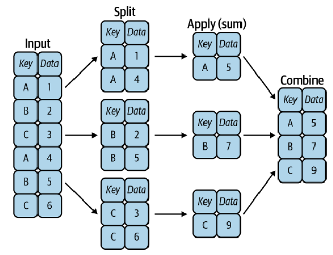
Fig. 4.1 A visual representation of a groupby operation [Vanderplas, 2022]#
4.5.2.2.1. GroupBy Workflow: From Split to Results#
Understanding GroupBy operations requires grasping the split-apply-combine workflow that happens behind the scenes. When you call df.groupby('column'), you’re not getting results immediately: you’re creating a GroupBy object that represents your grouped data structure.
# Step 1: SPLIT - Create groups (no calculation yet)
grouped = df.groupby('category')
print(type(grouped))  # <class 'pandas.core.groupby.generic.DataFrameGroupBy'>

# Step 2: APPLY & COMBINE - Trigger calculation and combine results
result = grouped.sum()  # Now pandas computes sum for each group
Why this design matters:
Efficiency: Data is grouped once, then multiple operations can be applied
Flexibility: Same grouped structure can be used for different calculations
Readability: Natural method chaining like
df.groupby('region').sum().sort_values()
4.5.2.2.2. Essential GroupBy Methods#
Basic Statistics
Method |
Returns |
Best For |
Example |
|---|---|---|---|
|
Sum of each group |
Revenue totals |
|
|
Average of each group |
Performance averages |
|
|
Middle value of each group |
Typical values |
|
|
Smallest value in each group |
Best/worst performers |
|
|
Largest value in each group |
Peak performance |
|
|
Standard deviation |
Measuring variability |
|
Counting Operations
Method |
Returns |
Key Difference |
When to Use |
|---|---|---|---|
|
Non-null values |
Excludes NaN |
Count valid responses |
|
Total rows |
Includes NaN |
Count all observations |
|
Unique values |
Counts distinct items |
Count variety/diversity |
Selection Methods
Method |
Returns |
Typical Use Case |
|---|---|---|
|
First value in group |
Initial measurements, baseline data |
|
Last value in group |
Final status, most recent data |
Advanced Functions
Method |
Power Level |
Description |
Example Use |
|---|---|---|---|
|
Basic |
Apply multiple functions |
|
|
Intermediate |
Custom function per group |
Complex calculations, custom logic |
|
Advanced |
Same-size output |
Normalize within groups, percentage of group |
Power User Techniques
# Multi-function aggregation
sales_summary = df.groupby('region').agg({
    'revenue': ['sum', 'mean', 'count'],
    'customers': 'nunique',
    'orders': 'size'
})

# Method chaining for complex analysis
top_regions = (df.groupby('region')['revenue']
               .sum()
               .sort_values(ascending=False)
               .head(5))

# Transform for group-wise calculations
df['revenue_pct_of_region'] = (df['revenue'] /
                               df.groupby('region')['revenue'].transform('sum') * 100)
Critical Distinctions to Remember
.count()vs.size():.count()excludes NaN values,.size()includes them.agg()vs.apply():.agg()for standard functions,.apply()for custom logic.apply()vs.transform():.apply()can change output size,.transform()maintains original DataFrame dimensions
These methods form the foundation of sophisticated data analysis, enabling you to uncover patterns and insights that would be impossible to see in raw data.
data = {        ### create a dictionary with data

    'Company': ['GOOG', 'GOOG', 'MSFT', 'MSFT', 'FB', 'FB'],
    'Person': ['Sam', 'Charlie', 'Amy', 'Vanessa', 'Carl', 'Sarah'],
    'Sales': [200, 120, 340, 124, 243, 350]
}

df = pd.DataFrame(data)     ### create the dataframe
df
| Company | Person | Sales | |
|---|---|---|---|
| 0 | GOOG | Sam | 200 |
| 1 | GOOG | Charlie | 120 |
| 2 | MSFT | Amy | 340 |
| 3 | MSFT | Vanessa | 124 |
| 4 | FB | Carl | 243 |
| 5 | FB | Sarah | 350 |
Now you can use the .groupby() method to group rows together based off of a column name. For instance let’s group based off of Company. This will create a DataFrameGroupBy object:
df.groupby('Company')
<pandas.core.groupby.generic.DataFrameGroupBy object at 0x119b8f620>
You can save this object as a new variable:
by_comp = df.groupby("Company")
The idea of groupby becomes clear if you do a .describe on the object. Notice the data index now is grouped by company.
by_comp.describe()
| Sales | ||||||||
|---|---|---|---|---|---|---|---|---|
| count | mean | std | min | 25% | 50% | 75% | max | |
| Company | ||||||||
| FB | 2.0 | 296.5 | 75.660426 | 243.0 | 269.75 | 296.5 | 323.25 | 350.0 |
| GOOG | 2.0 | 160.0 | 56.568542 | 120.0 | 140.00 | 160.0 | 180.00 | 200.0 |
| MSFT | 2.0 | 232.0 | 152.735065 | 124.0 | 178.00 | 232.0 | 286.00 | 340.0 |
And then call aggregate methods off the object:
by_comp['Sales'].mean() ### by_comp.mean()
Company
FB      296.5
GOOG    160.0
MSFT    232.0
Name: Sales, dtype: float64
Or you may just chain the methods together.
df.groupby('Company')['Sales'].mean()
Company
FB      296.5
GOOG    160.0
MSFT    232.0
Name: Sales, dtype: float64
More examples of aggregate methods:
by_comp["Sales"].std()
Company
FB       75.660426
GOOG     56.568542
MSFT    152.735065
Name: Sales, dtype: float64
by_comp.min()
| Person | Sales | |
|---|---|---|
| Company | ||
| FB | Carl | 243 |
| GOOG | Charlie | 120 |
| MSFT | Amy | 124 |
by_comp.max()
| Person | Sales | |
|---|---|---|
| Company | ||
| FB | Sarah | 350 |
| GOOG | Sam | 200 |
| MSFT | Vanessa | 340 |
by_comp.count()
| Person | Sales | |
|---|---|---|
| Company | ||
| FB | 2 | 2 |
| GOOG | 2 | 2 |
| MSFT | 2 | 2 |
by_comp.describe().transpose()
| Company | FB | GOOG | MSFT | |
|---|---|---|---|---|
| Sales | count | 2.000000 | 2.000000 | 2.000000 |
| mean | 296.500000 | 160.000000 | 232.000000 | |
| std | 75.660426 | 56.568542 | 152.735065 | |
| min | 243.000000 | 120.000000 | 124.000000 | |
| 25% | 269.750000 | 140.000000 | 178.000000 | |
| 50% | 296.500000 | 160.000000 | 232.000000 | |
| 75% | 323.250000 | 180.000000 | 286.000000 | |
| max | 350.000000 | 200.000000 | 340.000000 |
by_comp.describe().transpose()['GOOG']
Sales  count      2.000000
       mean     160.000000
       std       56.568542
       min      120.000000
       25%      140.000000
       50%      160.000000
       75%      180.000000
       max      200.000000
Name: GOOG, dtype: float64
### EXERCISE: GroupBy Operations
#
# 1. print: Use the company sales data ("df") from the data:
#           {'Company': ['GOOG', 'GOOG', 'MSFT', 'MSFT', 'FB', 'FB'],
#               'Person': ['Sam', 'Charlie', 'Amy', 'Vanessa', 'Carl', 'Sarah'],
#               'Sales': [200, 120, 340, 124, 243, 350]}
# 2. print: Group by Company and calculate the total sales for each company
# 3. print: Group by Company and find the maximum sales for each company
# 4. print: Group by Company and count how many salespeople each company has
#
### Your code starts here:


### Your code ends here.
Original DataFrame:
  Company   Person  Sales
0    GOOG      Sam    200
1    GOOG  Charlie    120
2    MSFT      Amy    340
3    MSFT  Vanessa    124
4      FB     Carl    243
5      FB    Sarah    350

Total sales per company:
Company
FB      593
GOOG    320
MSFT    464
Name: Sales, dtype: int64

Maximum sales per company:
Company
FB      350
GOOG    200
MSFT    340
Name: Sales, dtype: int64

Number of salespeople per company:
Company
FB      2
GOOG    2
MSFT    2
Name: Person, dtype: int64
4.5.3. Applying Functions: map() and apply()#
Two of the most frequently used pandas tools for transforming data are map() and apply(). Both let you run a function on your data without writing an explicit loop, but they work at different levels:
Method |
Works on |
Applies function to |
Typical use |
|---|---|---|---|
|
Series (one column) |
Each element |
Encode/translate values, simple element-wise transforms |
|
DataFrame or Series |
Each column (default) or each row |
Column-level calculations, combining columns |
4.5.3.1. Series.map()#
map() transforms every element in a Series. You can pass:
a function (or lambda)
a dictionary that maps old values to new values
another Series to look values up in
# Rebuild the company-sales DataFrame used in the GroupBy section
df = pd.DataFrame({
    'Company': ['GOOG', 'GOOG', 'MSFT', 'MSFT', 'FB', 'FB'],
    'Person':  ['Sam', 'Charlie', 'Amy', 'Vanessa', 'Carl', 'Sarah'],
    'Sales':   [200, 120, 340, 124, 243, 350]
})

# --- map() with a dictionary ---
# Translate abbreviated company names to full names
name_map = {'GOOG': 'Google', 'MSFT': 'Microsoft', 'FB': 'Meta'}
df['Company_Full'] = df['Company'].map(name_map)
df
| Company | Person | Sales | Company_Full | |
|---|---|---|---|---|
| 0 | GOOG | Sam | 200 | |
| 1 | GOOG | Charlie | 120 | |
| 2 | MSFT | Amy | 340 | Microsoft |
| 3 | MSFT | Vanessa | 124 | Microsoft |
| 4 | FB | Carl | 243 | Meta |
| 5 | FB | Sarah | 350 | Meta |
# --- map() with a lambda ---
# Categorize sales as 'High' (>= 200) or 'Low' (< 200) using a lambda
df['Sales_Tier'] = df['Sales'].map(lambda x: 'High' if x >= 200 else 'Low')
df
| Company | Person | Sales | Company_Full | Sales_Tier | |
|---|---|---|---|---|---|
| 0 | GOOG | Sam | 200 | High | |
| 1 | GOOG | Charlie | 120 | Low | |
| 2 | MSFT | Amy | 340 | Microsoft | High |
| 3 | MSFT | Vanessa | 124 | Microsoft | Low |
| 4 | FB | Carl | 243 | Meta | High |
| 5 | FB | Sarah | 350 | Meta | High |
4.5.3.2. df.apply()#
apply() passes each column (or row when axis=1) to a function and collects the results. This makes it easy to run custom calculations that span multiple cells without writing a loop.
df.apply(func)           # applies func to each column (returns a Series per column)
df.apply(func, axis=1)   # applies func to each row
# Retail orders: Revenue, Cost, and Units sold per transaction
orders = pd.DataFrame({
    'Revenue':  [1200, 450, 3200, 870, 2100, 640],
    'Cost':     [ 800, 310, 2100, 590, 1400, 420],
    'Units':    [   3,   2,    8,   3,    5,   2]
}, index=['Ord-001', 'Ord-002', 'Ord-003', 'Ord-004', 'Ord-005', 'Ord-006'])

# apply() column-wise (axis=0, default): spread (max − min) of each metric
print(f"{orders}\n")

orders['Profit/Unit'] = orders.apply(lambda row: round((row["Revenue"] - row["Cost"]) / row["Units"], 2), axis=1)
print(orders)
         Revenue  Cost  Units
Ord-001     1200   800      3
Ord-002      450   310      2
Ord-003     3200  2100      8
Ord-004      870   590      3
Ord-005     2100  1400      5
Ord-006      640   420      2

         Revenue  Cost  Units  Profit/Unit
Ord-001     1200   800      3       133.33
Ord-002      450   310      2        70.00
Ord-003     3200  2100      8       137.50
Ord-004      870   590      3        93.33
Ord-005     2100  1400      5       140.00
Ord-006      640   420      2       110.00
# apply() row-wise (axis=1): calculate profit per order
orders['Profit'] = orders.apply(lambda row: row['Revenue'] - row['Cost'], axis=1)

# apply() with a named function — classify order size by revenue
def order_tier(row):
    if row['Revenue'] >= 2000:
        return 'Large'
    elif row['Revenue'] >= 1000:
        return 'Medium'
    else:
        return 'Small'

orders['Tier'] = orders.apply(order_tier, axis=1)
orders
| Revenue | Cost | Units | Profit/Unit | Profit | Tier | |
|---|---|---|---|---|---|---|
| Ord-001 | 1200 | 800 | 3 | 133.33 | 400.0 | Medium |
| Ord-002 | 450 | 310 | 2 | 70.00 | 140.0 | Small |
| Ord-003 | 3200 | 2100 | 8 | 137.50 | 1100.0 | Large |
| Ord-004 | 870 | 590 | 3 | 93.33 | 280.0 | Small |
| Ord-005 | 2100 | 1400 | 5 | 140.00 | 700.0 | Large |
| Ord-006 | 640 | 420 | 2 | 110.00 | 220.0 | Small |
4.5.3.2.1. apply() with groupby()#
apply() is especially powerful when combined with groupby(). It lets you run any custom function on each group — not just the built-in aggregations like sum() or mean().
# Rebuild the sales DataFrame (Company_Full and Sales_Tier columns not needed here)
df_sales = pd.DataFrame({
    'Company': ['GOOG', 'GOOG', 'MSFT', 'MSFT', 'FB', 'FB'],
    'Person':  ['Sam', 'Charlie', 'Amy', 'Vanessa', 'Carl', 'Sarah'],
    'Sales':   [200, 120, 340, 124, 243, 350]
})

# Custom function: normalize Sales within each company group
# (each value minus group mean, divided by group std)
def normalize(group):
    return (group - group.mean()) / group.std()

df_sales['Sales_Normalized'] = df_sales.groupby('Company')['Sales'].apply(normalize).reset_index(level=0, drop=True)
df_sales
| Company | Person | Sales | Sales_Normalized | |
|---|---|---|---|---|
| 0 | GOOG | Sam | 200 | 0.707107 |
| 1 | GOOG | Charlie | 120 | -0.707107 |
| 2 | MSFT | Amy | 340 | 0.707107 |
| 3 | MSFT | Vanessa | 124 | -0.707107 |
| 4 | FB | Carl | 243 | -0.707107 |
| 5 | FB | Sarah | 350 | 0.707107 |
### EXERCISE: map() and apply()
#
# Given this employee DataFrame:
emp = pd.DataFrame({
    'Name':       ['Alice', 'Bob', 'Carol', 'Dave'],
    'Department': ['Eng', 'HR', 'Eng', 'HR'],
    'Salary':     [95000, 62000, 105000, 58000]
})
#
# Tasks:
# 1. Use map() with a dictionary to add a 'Dept_Full' column that expands
#    'Eng' → 'Engineering' and 'HR' → 'Human Resources'
# 2. Use apply() (column-wise, axis=0) to print the max salary in each numeric column
# 3. Use apply() (row-wise, axis=1) to add a 'Bonus' column:
#    10 % of Salary for Engineering employees, 8 % for all others
#
### Your code starts here:


### Your code ends here.
# Solution

emp = pd.DataFrame({
    'Name':       ['Alice', 'Bob', 'Carol', 'Dave'],
    'Department': ['Eng', 'HR', 'Eng', 'HR'],
    'Salary':     [95000, 62000, 105000, 58000]
})

# 1. map() with a dictionary
dept_map = {'Eng': 'Engineering', 'HR': 'Human Resources'}
emp['Dept_Full'] = emp['Department'].map(dept_map)
print("1. Dept_Full column added via map():")
print(emp)
print()

# 2. apply() column-wise — max of each numeric column
print("2. Column max via apply():")
print(emp[['Salary']].apply(lambda col: col.max()))
print()

# 3. apply() row-wise — compute bonus
def calc_bonus(row):
    rate = 0.10 if row['Department'] == 'Eng' else 0.08
    return row['Salary'] * rate

emp['Bonus'] = emp.apply(calc_bonus, axis=1)
print("3. Bonus column added via apply():")
print(emp)
1. Dept_Full column added via map():
    Name Department  Salary        Dept_Full
0  Alice        Eng   95000      Engineering
1    Bob         HR   62000  Human Resources
2  Carol        Eng  105000      Engineering
3   Dave         HR   58000  Human Resources

2. Column max via apply():
Salary    105000
dtype: int64

3. Bonus column added via apply():
    Name Department  Salary        Dept_Full    Bonus
0  Alice        Eng   95000      Engineering   9500.0
1    Bob         HR   62000  Human Resources   4960.0
2  Carol        Eng  105000      Engineering  10500.0
3   Dave         HR   58000  Human Resources   4640.0
4.5.4. DataFrame Operations#
Raw data is rarely in the perfect form for analysis. Real-world datasets often need cleaning, organizing, and restructuring before meaningful insights can be extracted. This section explores essential DataFrame manipulation operations that help transform messy data into analysis-ready formats.
We’ll cover three fundamental operations that every data analyst should master:
Sorting: Arranging data in meaningful order to reveal patterns and facilitate analysis
Handling Duplicates: Identifying and managing redundant records that can skew results
Renaming: Creating clear, descriptive labels that improve code readability and collaboration
These operations form the foundation of data preprocessing and are crucial steps in any data analysis workflow.
4.5.4.1. Sorting#
### Recreate DataFrame with random data for sorting examples
np.random.seed(42)
dates = pd.date_range('20250901', periods=5)
df_sort = pd.DataFrame(np.random.randn(5, 4), index=dates, columns=list('WXYZ'))
df_sort
| W | X | Y | Z | |
|---|---|---|---|---|
| 2025-09-01 | 0.496714 | -0.138264 | 0.647689 | 1.523030 |
| 2025-09-02 | -0.234153 | -0.234137 | 1.579213 | 0.767435 |
| 2025-09-03 | -0.469474 | 0.542560 | -0.463418 | -0.465730 |
| 2025-09-04 | 0.241962 | -1.913280 | -1.724918 | -0.562288 |
| 2025-09-05 | -1.012831 | 0.314247 | -0.908024 | -1.412304 |
# Sort by a single column (ascending)
df_sort.sort_values(by='W')
| W | X | Y | Z | |
|---|---|---|---|---|
| 2025-09-05 | -1.012831 | 0.314247 | -0.908024 | -1.412304 |
| 2025-09-03 | -0.469474 | 0.542560 | -0.463418 | -0.465730 |
| 2025-09-02 | -0.234153 | -0.234137 | 1.579213 | 0.767435 |
| 2025-09-04 | 0.241962 | -1.913280 | -1.724918 | -0.562288 |
| 2025-09-01 | 0.496714 | -0.138264 | 0.647689 | 1.523030 |
# Sort by multiple columns
df_sort.sort_values(by=['W', 'Z'])
| W | X | Y | Z | |
|---|---|---|---|---|
| 2025-09-05 | -1.012831 | 0.314247 | -0.908024 | -1.412304 |
| 2025-09-03 | -0.469474 | 0.542560 | -0.463418 | -0.465730 |
| 2025-09-02 | -0.234153 | -0.234137 | 1.579213 | 0.767435 |
| 2025-09-04 | 0.241962 | -1.913280 | -1.724918 | -0.562288 |
| 2025-09-01 | 0.496714 | -0.138264 | 0.647689 | 1.523030 |
# Sort by index labels
df_sort.sort_index()
| W | X | Y | Z | |
|---|---|---|---|---|
| 2025-09-01 | 0.496714 | -0.138264 | 0.647689 | 1.523030 |
| 2025-09-02 | -0.234153 | -0.234137 | 1.579213 | 0.767435 |
| 2025-09-03 | -0.469474 | 0.542560 | -0.463418 | -0.465730 |
| 2025-09-04 | 0.241962 | -1.913280 | -1.724918 | -0.562288 |
| 2025-09-05 | -1.012831 | 0.314247 | -0.908024 | -1.412304 |
4.5.4.1.1. inplace=True#
By default, sort_values() and sort_index() return a new DataFrame and do not modify the original. There are two ways to make the sort permanent:
Option 1 — Reassignment (recommended):
df_sort = df_sort.sort_values(by='W')
Option 2 — inplace=True:
df_sort.sort_values(by='W', inplace=True)
Both approaches produce the same result. Reassignment is generally preferred in modern pandas because it is more explicit and avoids subtle bugs in chained operations.
# Show that sort_values does NOT change the original by default
print("Before sort:")
print(df_sort)

result = df_sort.sort_values(by='W')   # returns a new DataFrame
print("\nAfter sort_values (original df_sort unchanged):")
print(df_sort)

# Option 1: reassignment
df_sort_v1 = df_sort.sort_values(by='W')
print("\nOption 1 — reassignment (df_sort_v1):")
print(df_sort_v1)

# Option 2: inplace=True
df_sort_v2 = df_sort.copy()            # copy so we preserve df_sort for the rest of the notebook
df_sort_v2.sort_values(by='W', inplace=True)
print("\nOption 2 — inplace=True (df_sort_v2):")
print(df_sort_v2)
Before sort:
                   W         X         Y         Z
2025-09-01  0.496714 -0.138264  0.647689  1.523030
2025-09-02 -0.234153 -0.234137  1.579213  0.767435
2025-09-03 -0.469474  0.542560 -0.463418 -0.465730
2025-09-04  0.241962 -1.913280 -1.724918 -0.562288
2025-09-05 -1.012831  0.314247 -0.908024 -1.412304

After sort_values (original df_sort unchanged):
                   W         X         Y         Z
2025-09-01  0.496714 -0.138264  0.647689  1.523030
2025-09-02 -0.234153 -0.234137  1.579213  0.767435
2025-09-03 -0.469474  0.542560 -0.463418 -0.465730
2025-09-04  0.241962 -1.913280 -1.724918 -0.562288
2025-09-05 -1.012831  0.314247 -0.908024 -1.412304

Option 1 — reassignment (df_sort_v1):
                   W         X         Y         Z
2025-09-05 -1.012831  0.314247 -0.908024 -1.412304
2025-09-03 -0.469474  0.542560 -0.463418 -0.465730
2025-09-02 -0.234153 -0.234137  1.579213  0.767435
2025-09-04  0.241962 -1.913280 -1.724918 -0.562288
2025-09-01  0.496714 -0.138264  0.647689  1.523030

Option 2 — inplace=True (df_sort_v2):
                   W         X         Y         Z
2025-09-05 -1.012831  0.314247 -0.908024 -1.412304
2025-09-03 -0.469474  0.542560 -0.463418 -0.465730
2025-09-02 -0.234153 -0.234137  1.579213  0.767435
2025-09-04  0.241962 -1.913280 -1.724918 -0.562288
2025-09-01  0.496714 -0.138264  0.647689  1.523030
### EXERCISE: Sorting DataFrames
import pandas as pd
# Create a DataFrame:
sort_df = pd.DataFrame({
    'Name': ['Alice', 'Bob', 'Charlie', 'Diana'],
    'Age': [25, 30, 22, 28],
    'Score': [85, 92, 78, 92]
})
#
# Tasks:
# 1. Sort by Age in ascending order
# 2. Sort by Score in descending order
# 3. Sort by Score (descending), then by Age (ascending)
# 4. Sort by index
#
### Your code starts here:


### Your code ends here.
1. Sort by Age in ascending order:
      Name  Age  Score
2  Charlie   22     78
0    Alice   25     85
3    Diana   28     92
1      Bob   30     92

2. Sort by Score in descending order:
      Name  Age  Score
1      Bob   30     92
3    Diana   28     92
0    Alice   25     85
2  Charlie   22     78

3. Sort by Score (descending), then by Age (ascending):
      Name  Age  Score
3    Diana   28     92
1      Bob   30     92
0    Alice   25     85
2  Charlie   22     78

4. Sort by index:       Name  Age  Score
0    Alice   25     85
1      Bob   30     92
2  Charlie   22     78
3    Diana   28     92
4.5.4.2. Handling Duplicates#
DataFrames often contain duplicate rows. Pandas provides methods to identify and remove them.
# Create a DataFrame with duplicate rows for demonstration
df_dup = pd.DataFrame({
    'A': [1, 2, 2, 3, 3, 4],
    'B': [10, 20, 20, 30, 30, 40],
    'C': ['x', 'y', 'y', 'z', 'w', 'v']
})
df_dup
| A | B | C | |
|---|---|---|---|
| 0 | 1 | 10 | x |
| 1 | 2 | 20 | y |
| 2 | 2 | 20 | y |
| 3 | 3 | 30 | z |
| 4 | 3 | 30 | w |
| 5 | 4 | 40 | v |
# Check for duplicate rows (returns boolean Series)
df_dup.duplicated()
0    False
1    False
2     True
3    False
4    False
5    False
dtype: bool
# Drop duplicates based on specific columns
df_dup.drop_duplicates(subset=['A'])
| A | B | C | |
|---|---|---|---|
| 0 | 1 | 10 | x |
| 1 | 2 | 20 | y |
| 3 | 3 | 30 | z |
| 5 | 4 | 40 | v |
### EXERCISE: Working with Duplicates
#
# Create a DataFrame:
dup_df = pd.DataFrame({
    'A': [1, 2, 2, 3, 3, 4],
    'B': [10, 20, 20, 30, 30, 40],
    'C': ['x', 'y', 'y', 'z', 'w', 'v']
})
#
# Tasks:
# 1. Display the DataFrame
# 2. Check for duplicates (use .duplicated())
# 3. Remove all duplicates (use .drop_duplicates())
# 4. Remove duplicates based on column A only
#
### Your code starts here:


### Your code ends here.
Original DataFrame:
   A   B  C
0  1  10  x
1  2  20  y
2  2  20  y
3  3  30  z
4  3  30  w
5  4  40  v

Duplicate rows:
0    False
1    False
2     True
3    False
4    False
5    False
dtype: bool

After removing all duplicates:
   A   B  C
0  1  10  x
1  2  20  y
3  3  30  z
4  3  30  w
5  4  40  v

After removing duplicates in column A:
   A   B  C
0  1  10  x
1  2  20  y
3  3  30  z
5  4  40  v
4.5.4.3. Renaming Columns and Index#
Pandas provides the .rename() method to rename columns and index labels. This is useful when you need more descriptive names or want to standardize naming conventions.
Let’s start with our sample DataFrame:
df_sort
| W | X | Y | Z | |
|---|---|---|---|---|
| 2025-09-01 | 0.496714 | -0.138264 | 0.647689 | 1.523030 |
| 2025-09-02 | -0.234153 | -0.234137 | 1.579213 | 0.767435 |
| 2025-09-03 | -0.469474 | 0.542560 | -0.463418 | -0.465730 |
| 2025-09-04 | 0.241962 | -1.913280 | -1.724918 | -0.562288 |
| 2025-09-05 | -1.012831 | 0.314247 | -0.908024 | -1.412304 |
# Rename columns
df_sort.rename(columns={'W': 'Weight', 'X': 'X_coord'})
| Weight | X_coord | Y | Z | |
|---|---|---|---|---|
| 2025-09-01 | 0.496714 | -0.138264 | 0.647689 | 1.523030 |
| 2025-09-02 | -0.234153 | -0.234137 | 1.579213 | 0.767435 |
| 2025-09-03 | -0.469474 | 0.542560 | -0.463418 | -0.465730 |
| 2025-09-04 | 0.241962 | -1.913280 | -1.724918 | -0.562288 |
| 2025-09-05 | -1.012831 | 0.314247 | -0.908024 | -1.412304 |
4.5.4.3.1. inplace=True with rename()#
Like sort_values(), rename() also returns a new DataFrame by default — the original is not modified. Apply the same two options:
Option 1 — Reassignment (recommended):
df_sort = df_sort.rename(columns={'W': 'Weight', 'X': 'X_coord'})
Option 2 — inplace=True:
df_sort.rename(columns={'W': 'Weight', 'X': 'X_coord'}, inplace=True)
# rename() does NOT change df_sort by default
print("Before rename:")
print(df_sort)

df_sort.rename(columns={'W': 'Weight', 'X': 'X_coord'})  # result discarded — df_sort unchanged
print("\nAfter rename() without assignment (df_sort unchanged):")
print(df_sort)

# Option 1: reassignment
df_renamed = df_sort.rename(columns={'W': 'Weight', 'X': 'X_coord'})
print("\nOption 1 — reassignment (df_renamed):")
print(df_renamed)

# Option 2: inplace=True
df_inplace = df_sort.copy()
df_inplace.rename(columns={'W': 'Weight', 'X': 'X_coord'}, inplace=True)
print("\nOption 2 — inplace=True (df_inplace):")
print(df_inplace)
Before rename:
                   W         X         Y         Z
2025-09-01  0.496714 -0.138264  0.647689  1.523030
2025-09-02 -0.234153 -0.234137  1.579213  0.767435
2025-09-03 -0.469474  0.542560 -0.463418 -0.465730
2025-09-04  0.241962 -1.913280 -1.724918 -0.562288
2025-09-05 -1.012831  0.314247 -0.908024 -1.412304

After rename() without assignment (df_sort unchanged):
                   W         X         Y         Z
2025-09-01  0.496714 -0.138264  0.647689  1.523030
2025-09-02 -0.234153 -0.234137  1.579213  0.767435
2025-09-03 -0.469474  0.542560 -0.463418 -0.465730
2025-09-04  0.241962 -1.913280 -1.724918 -0.562288
2025-09-05 -1.012831  0.314247 -0.908024 -1.412304

Option 1 — reassignment (df_renamed):
              Weight   X_coord         Y         Z
2025-09-01  0.496714 -0.138264  0.647689  1.523030
2025-09-02 -0.234153 -0.234137  1.579213  0.767435
2025-09-03 -0.469474  0.542560 -0.463418 -0.465730
2025-09-04  0.241962 -1.913280 -1.724918 -0.562288
2025-09-05 -1.012831  0.314247 -0.908024 -1.412304

Option 2 — inplace=True (df_inplace):
              Weight   X_coord         Y         Z
2025-09-01  0.496714 -0.138264  0.647689  1.523030
2025-09-02 -0.234153 -0.234137  1.579213  0.767435
2025-09-03 -0.469474  0.542560 -0.463418 -0.465730
2025-09-04  0.241962 -1.913280 -1.724918 -0.562288
2025-09-05 -1.012831  0.314247 -0.908024 -1.412304
### EXERCISE: Renaming DataFrame Elements
#
# Create a DataFrame:
rename_df = pd.DataFrame({
    'a': [1, 2, 3],
    'b': [4, 5, 6],
    'c': [7, 8, 9]
}, index=['row1', 'row2', 'row3'])
#
# Tasks:
# 1. Display the original DataFrame
# 2. Rename column 'a' to 'Alpha' and 'b' to 'Beta'
# 3. Rename the index 'row1' to 'R1' and 'row2' to 'R2'
# 4. Display the renamed DataFrame
#
### Your code starts here:


### Your code ends here.
Original DataFrame:
      a  b  c
row1  1  4  7
row2  2  5  8
row3  3  6  9

Renamed DataFrame:
      Alpha  Beta  c
R1        1     4  7
R2        2     5  8
row3      3     6  9
# Flexible display_side_by_side function that handles both calling patterns
from IPython.display import HTML
import pandas as pd

def display_side_by_side(*args, names=None):
    """
    Display DataFrames side by side using HTML formatting.
    Handles both calling patterns:
    1. display_side_by_side(df1, df2, names=["Name1", "Name2"])
    2. display_side_by_side(df1, df2, "Name1", "Name2")
    """
    # Separate DataFrames from potential string names
    dfs = []
    string_names = []

    for arg in args:
        if isinstance(arg, (pd.DataFrame, pd.Series)):
            dfs.append(arg)
        elif isinstance(arg, str):
            string_names.append(arg)

    # Use provided names or string arguments or generate defaults
    if names is not None:
        final_names = names
    elif string_names:
        final_names = string_names
    else:
        final_names = [f'DataFrame {i+1}' for i in range(len(dfs))]

    # Ensure we have enough names
    while len(final_names) < len(dfs):
        final_names.append(f'DataFrame {len(final_names)+1}')

    html_str = '<div style="display: flex; gap: 20px;">'
    for df, name in zip(dfs, final_names):
        html_str += f'''
        <div>
            <h4>{name}</h4>
            {df.to_html()}
        </div>
        '''
    html_str += '</div>'
    return HTML(html_str)