9.6. Aggregation and groupby#
The groupby method allows you to group rows of data together and call aggregate functions
Efficient summarization is the core of data analysis. Aggregations (such as sum, mean, median, minimum, and maximum) compress key properties of datasets into single values, which can provide significant insights into data when conducting exploratory data analysis. This section examines aggregation in Pandas, starting with array-like operations comparable to those in NumPy, and advancing to more powerful techniques built on grouping (the concept of groupby).
import numpy as np
import pandas as pd
9.6.1. Simple Aggregations#
Now we can start with reviewing some simple aggregations on random values using NumPy and Pandas, e.g., sum and mean. Note that these operations return single values.
### let's use NumPy's new random API to generate some random numbers

### create a random number generator with a fixed SEED for reproducibility
rng = np.random.default_rng(42)
ser = pd.Series(rng.integers(0, 10, 5))
ser
0    0
1    7
2    6
3    4
4    4
dtype: int64
### sum
print(ser.sum())
21
### mean
print(ser.mean())
4.2
Now let’s try a few more aggregations on a DataFrame.
### create a DataFrame with random numbers for two columns 'A' and 'B'
### using the same random number generator
### note this is a dictionary where keys are column names and
### values are sequences (lists/arrays/range) of data

rng = np.random.default_rng(42)
df = pd.DataFrame(
    {
     'A': rng.random(5),
     'B': rng.random(5)
     }
)
df
| A | B | |
|---|---|---|
| 0 | 0.773956 | 0.975622 |
| 1 | 0.438878 | 0.761140 |
| 2 | 0.858598 | 0.786064 |
| 3 | 0.697368 | 0.128114 |
| 4 | 0.094177 | 0.450386 |
df.mean() ### mean for each column
A    0.572596
B    0.620265
dtype: float64
df.sum() ### sum for each column
A    2.862978
B    3.101326
dtype: float64
Now, we’ll start with loading the Planets dataset (which is available through the Seaborn visualization package and will be covered later). This dataset has details about more than one thousand extrasolar planets discovered up to 2014.
### more than likely you have not installed seaborn
### you can do so by running the following command in your terminal
### pip install seaborn
### or uncomment the following line to install via pip directly in the notebook

# %pip install seaborn

### don't forget to comment it back out after installation
### run this cell to load the dataset

import seaborn as sns
planets = sns.load_dataset('planets')   ### syntax to load a dataset from seaborn
### check out the first few rows of the dataset

planets.head()
| method | number | orbital_period | mass | distance | year | |
|---|---|---|---|---|---|---|
| 0 | Radial Velocity | 1 | 269.300 | 7.10 | 77.40 | 2006 |
| 1 | Radial Velocity | 1 | 874.774 | 2.21 | 56.95 | 2008 |
| 2 | Radial Velocity | 1 | 763.000 | 2.60 | 19.84 | 2011 |
| 3 | Radial Velocity | 1 | 326.030 | 19.40 | 110.62 | 2007 |
| 4 | Radial Velocity | 1 | 516.220 | 10.50 | 119.47 | 2009 |
Aggregation methods work similarly/the same. Here’s a list of Pandas aggregation methods.
Aggregation |
Returns |
|---|---|
count |
Total number of items |
first, last |
First and last item |
mean, median |
Mean and median |
min, max |
Minimum and maximum |
std, var |
Standard deviation and variance |
mad |
Mean absolute deviation |
prod |
Product of all items |
sum |
Sum of all items |
9.6.2. groupby#
While simple aggregations provide a quick overview of a dataset, analyses often require conditional aggregation by category or index level. In Pandas, this is accomplished with the groupby operation. The term originates from SQL’s GROUP BY, but conceptually it follows Hadley Wickham’s split–apply–combine paradigm: split the data into groups, apply a function to each group, and combine the results into a single output groupby.
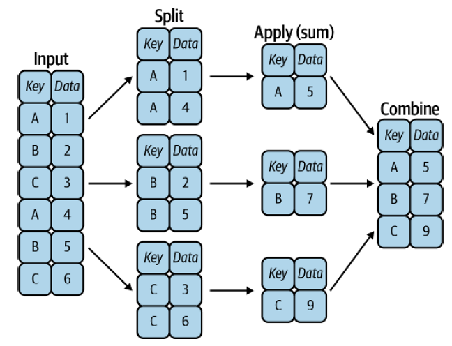
Fig. 9.1 A visual representation of a groupby operation [Vanderplas, 2022]#
### create sample dataframe
### start with a dictionary

data = {
    'Company': ['GOOG', 'GOOG', 'MSFT', 'MSFT', 'FB', 'FB'],
    'Person': ['Sam', 'Charlie', 'Amy', 'Vanessa', 'Carl', 'Sarah'],
    'Sales': [200, 120, 340, 124, 243, 350]
}
### check out the data dictionary

data
{'Company': ['GOOG', 'GOOG', 'MSFT', 'MSFT', 'FB', 'FB'],
 'Person': ['Sam', 'Charlie', 'Amy', 'Vanessa', 'Carl', 'Sarah'],
 'Sales': [200, 120, 340, 124, 243, 350]}
### create the dataframe

df = pd.DataFrame(data)
df
| Company | Person | Sales | |
|---|---|---|---|
| 0 | GOOG | Sam | 200 |
| 1 | GOOG | Charlie | 120 |
| 2 | MSFT | Amy | 340 |
| 3 | MSFT | Vanessa | 124 |
| 4 | FB | Carl | 243 |
| 5 | FB | Sarah | 350 |
Now you can use the .groupby() method to group rows together based off of a column name. For instance let’s group based off of Company. This will create a DataFrameGroupBy object:
df.groupby('Company')
<pandas.core.groupby.generic.DataFrameGroupBy object at 0x10c2cb250>
You can save this object as a new variable:
by_comp = df.groupby("Company")
And then call aggregate methods off the object:
# by_comp.mean()
by_comp['Sales'].mean()
Company
FB      296.5
GOOG    160.0
MSFT    232.0
Name: Sales, dtype: float64
# df.groupby('Company').mean()
df.groupby('Company')['Sales'].mean()
Company
FB      296.5
GOOG    160.0
MSFT    232.0
Name: Sales, dtype: float64
More examples of aggregate methods:
by_comp['Sales'].std()
Company
FB       75.660426
GOOG     56.568542
MSFT    152.735065
Name: Sales, dtype: float64
by_comp.min()
| Person | Sales | |
|---|---|---|
| Company | ||
| FB | Carl | 243 |
| GOOG | Charlie | 120 |
| MSFT | Amy | 124 |
by_comp.max()
| Person | Sales | |
|---|---|---|
| Company | ||
| FB | Sarah | 350 |
| GOOG | Sam | 200 |
| MSFT | Vanessa | 340 |
by_comp.count()
| Person | Sales | |
|---|---|---|
| Company | ||
| FB | 2 | 2 |
| GOOG | 2 | 2 |
| MSFT | 2 | 2 |
by_comp.describe()
| Sales | ||||||||
|---|---|---|---|---|---|---|---|---|
| count | mean | std | min | 25% | 50% | 75% | max | |
| Company | ||||||||
| FB | 2.0 | 296.5 | 75.660426 | 243.0 | 269.75 | 296.5 | 323.25 | 350.0 |
| GOOG | 2.0 | 160.0 | 56.568542 | 120.0 | 140.00 | 160.0 | 180.00 | 200.0 |
| MSFT | 2.0 | 232.0 | 152.735065 | 124.0 | 178.00 | 232.0 | 286.00 | 340.0 |
by_comp.describe().transpose()
| Company | FB | GOOG | MSFT | |
|---|---|---|---|---|
| Sales | count | 2.000000 | 2.000000 | 2.000000 |
| mean | 296.500000 | 160.000000 | 232.000000 | |
| std | 75.660426 | 56.568542 | 152.735065 | |
| min | 243.000000 | 120.000000 | 124.000000 | |
| 25% | 269.750000 | 140.000000 | 178.000000 | |
| 50% | 296.500000 | 160.000000 | 232.000000 | |
| 75% | 323.250000 | 180.000000 | 286.000000 | |
| max | 350.000000 | 200.000000 | 340.000000 |
by_comp.describe().transpose()['GOOG']
Sales  count      2.000000
       mean     160.000000
       std       56.568542
       min      120.000000
       25%      140.000000
       50%      160.000000
       75%      180.000000
       max      200.000000
Name: GOOG, dtype: float64