20.6. Multiple Regression

Now that we have explored ways to use multiple attributes to predict a categorical variable, let us return to predicting a quantitative variable. Predicting a numerical quantity is called regression, and a commonly used method to use multiple attributes for regression is called multiple linear regression.

20.6.1. Home Prices

The following dataset of house prices and attributes was collected over several years for the city of Ames, Iowa. A description of the dataset appears online . We will focus only a subset of the columns. We will try to predict the sale price column from the other columns.

all_sales = pd.read_csv(path_data + 'house.csv')
# len(all_sales)
all_sales

	Order	PID	MS SubClass	MS Zoning	Lot Frontage	Lot Area	Street	Alley	Lot Shape	Land Contour	...	Pool Area	Pool QC	Fence	Misc Feature	Misc Val	Mo Sold	Yr Sold	Sale Type	Sale Condition	SalePrice
0	1	526301100	20	RL	141.0	31770	Pave	NaN	IR1	Lvl	...	0	NaN	NaN	NaN	0	5	2010	WD	Normal	215000
1	2	526350040	20	RH	80.0	11622	Pave	NaN	Reg	Lvl	...	0	NaN	MnPrv	NaN	0	6	2010	WD	Normal	105000
2	3	526351010	20	RL	81.0	14267	Pave	NaN	IR1	Lvl	...	0	NaN	NaN	Gar2	12500	6	2010	WD	Normal	172000
3	4	526353030	20	RL	93.0	11160	Pave	NaN	Reg	Lvl	...	0	NaN	NaN	NaN	0	4	2010	WD	Normal	244000
4	5	527105010	60	RL	74.0	13830	Pave	NaN	IR1	Lvl	...	0	NaN	MnPrv	NaN	0	3	2010	WD	Normal	189900
...	...	...	...	...	...	...	...	...	...	...	...	...	...	...	...	...	...	...	...	...	...
2925	2926	923275080	80	RL	37.0	7937	Pave	NaN	IR1	Lvl	...	0	NaN	GdPrv	NaN	0	3	2006	WD	Normal	142500
2926	2927	923276100	20	RL	NaN	8885	Pave	NaN	IR1	Low	...	0	NaN	MnPrv	NaN	0	6	2006	WD	Normal	131000
2927	2928	923400125	85	RL	62.0	10441	Pave	NaN	Reg	Lvl	...	0	NaN	MnPrv	Shed	700	7	2006	WD	Normal	132000
2928	2929	924100070	20	RL	77.0	10010	Pave	NaN	Reg	Lvl	...	0	NaN	NaN	NaN	0	4	2006	WD	Normal	170000
2929	2930	924151050	60	RL	74.0	9627	Pave	NaN	Reg	Lvl	...	0	NaN	NaN	NaN	0	11	2006	WD	Normal	188000

2930 rows × 82 columns

all_sales.describe()

	Order	PID	MS SubClass	Lot Frontage	Lot Area	Overall Qual	Overall Cond	Year Built	Year Remod/Add	Mas Vnr Area	...	Wood Deck SF	Open Porch SF	Enclosed Porch	3Ssn Porch	Screen Porch	Pool Area	Misc Val	Mo Sold	Yr Sold	SalePrice
count	2930.00000	2.930000e+03	2930.000000	2440.000000	2930.000000	2930.000000	2930.000000	2930.000000	2930.000000	2907.000000	...	2930.000000	2930.000000	2930.000000	2930.000000	2930.000000	2930.000000	2930.000000	2930.000000	2930.000000	2930.000000
mean	1465.50000	7.144645e+08	57.387372	69.224590	10147.921843	6.094881	5.563140	1971.356314	1984.266553	101.896801	...	93.751877	47.533447	23.011604	2.592491	16.002048	2.243345	50.635154	6.216041	2007.790444	180796.060068
std	845.96247	1.887308e+08	42.638025	23.365335	7880.017759	1.411026	1.111537	30.245361	20.860286	179.112611	...	126.361562	67.483400	64.139059	25.141331	56.087370	35.597181	566.344288	2.714492	1.316613	79886.692357
min	1.00000	5.263011e+08	20.000000	21.000000	1300.000000	1.000000	1.000000	1872.000000	1950.000000	0.000000	...	0.000000	0.000000	0.000000	0.000000	0.000000	0.000000	0.000000	1.000000	2006.000000	12789.000000
25%	733.25000	5.284770e+08	20.000000	58.000000	7440.250000	5.000000	5.000000	1954.000000	1965.000000	0.000000	...	0.000000	0.000000	0.000000	0.000000	0.000000	0.000000	0.000000	4.000000	2007.000000	129500.000000
50%	1465.50000	5.354536e+08	50.000000	68.000000	9436.500000	6.000000	5.000000	1973.000000	1993.000000	0.000000	...	0.000000	27.000000	0.000000	0.000000	0.000000	0.000000	0.000000	6.000000	2008.000000	160000.000000
75%	2197.75000	9.071811e+08	70.000000	80.000000	11555.250000	7.000000	6.000000	2001.000000	2004.000000	164.000000	...	168.000000	70.000000	0.000000	0.000000	0.000000	0.000000	0.000000	8.000000	2009.000000	213500.000000
max	2930.00000	1.007100e+09	190.000000	313.000000	215245.000000	10.000000	9.000000	2010.000000	2010.000000	1600.000000	...	1424.000000	742.000000	1012.000000	508.000000	576.000000	800.000000	17000.000000	12.000000	2010.000000	755000.000000

8 rows × 39 columns

sales1 = all_sales[all_sales['Bldg Type'] == '1Fam']
sales2 = sales1[sales1['Sale Condition'] == 'Normal']

sales = sales2[['SalePrice', '1st Flr SF', '2nd Flr SF', 
    'Total Bsmt SF', 'Garage Area', 
    'Wood Deck SF', 'Open Porch SF', 'Lot Area', 
    'Year Built', 'Yr Sold']]

sales = sales.sort_values(by=['SalePrice'])

len(sales)

2002

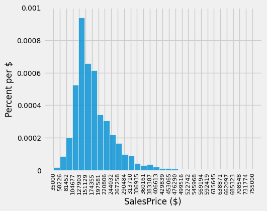
A histogram of sale prices shows a large amount of variability and a distribution that is clearly not normal. A long tail to the right contains a few houses that had very high prices. The short left tail does not contain any houses that sold for less than $35,000.

fig, ax = plt.subplots(figsize=(5,4))
ax.hist(sales['SalePrice'], bins=32, density=True, alpha=0.8, ec='white', zorder=5)

unit = '$'
y_label = 'Percent per ' + (unit if unit else 'unit')
x_label = 'SalesPrice ($)' 
plt.ylabel(y_label, fontsize=12)
plt.xlabel(x_label, fontsize=12)

x_min, x_max = sales['SalePrice'].min(), sales['SalePrice'].max()   ### multiple assignment
ax.set_xticks(np.linspace(x_min, x_max+.01, 32))
# ax.set_xticks(np.linspace(0, 800000, 9))

plt.xticks(rotation=90, fontsize=8)
plt.yticks(fontsize=10)

y_vals = ax.get_yticks()
ax.set_yticks(y_vals)
ax.set_yticklabels(['{:g}'.format(x * 100) for x in y_vals])

plt.title('');
plt.show()

20.6.1.1. Correlation

No single attribute is sufficient to predict the sale price. For example, the area of first floor, measured in square feet, correlates with sale price but only explains some of its variability.

fig, ax = plt.subplots(figsize=(5,4))

ax.scatter(
    sales['1st Flr SF'], 
    sales['SalePrice'],   
    color='darkblue', 
    alpha=0.8,
    s=5
)

x_label = '1st Flr SF'
y_label = 'SalePrice'

plt.ylabel(y_label)
plt.xlabel(x_label)
plt.show()

correlation(sales, 'SalePrice', '1st Flr SF')

0.6424662541030225

In fact, none of the individual attributes have a correlation with sale price that is above 0.7 (except for the sale price itself).

for label in sales.columns:
    print('Correlation of', label, 'and SalePrice:\t', correlation(sales, label, 'SalePrice'))

Correlation of SalePrice and SalePrice:	 1.0
Correlation of 1st Flr SF and SalePrice:	 0.6424662541030225
Correlation of 2nd Flr SF and SalePrice:	 0.3575218942800824
Correlation of Total Bsmt SF and SalePrice:	 0.652978626757169
Correlation of Garage Area and SalePrice:	 0.6385944852520442
Correlation of Wood Deck SF and SalePrice:	 0.3526986661950491
Correlation of Open Porch SF and SalePrice:	 0.3369094170263733
Correlation of Lot Area and SalePrice:	 0.29082345511576946
Correlation of Year Built and SalePrice:	 0.5651647537135916
Correlation of Yr Sold and SalePrice:	 0.025948579080721124

However, combining attributes can provide higher correlation. In particular, if we sum the first floor and second floor areas, the result has a higher correlation than any single attribute alone.

sales_copy = sales.copy()
both_floors = sales_copy.iloc[:,1] + sales_copy.iloc[:,2]

sales_copy['Both Floors'] = both_floors
correlation(sales_copy, 'SalePrice', 'Both Floors')

0.7821920556134877

# sales_copy.iloc[:,2]
# sales_copy['2nd Flr SF']

This high correlation indicates that we should try to use more than one attribute to predict the sale price. In a dataset with multiple observed attributes and a single numerical value to be predicted (the sale price in this case), multiple linear regression can be an effective technique.

20.6.2. Multiple Linear Regression

In multiple linear regression, a numerical output is predicted from numerical input attributes by multiplying each attribute value by a different slope, then summing the results. In this example, the slope for the 1st Flr SF would represent the dollars per square foot of area on the first floor of the house that should be used in our prediction.

Before we begin prediction, we split our data randomly into a training and test set of equal size.

20.6.2.1. Train/Test split

sales_copy = sales.copy()
train = sales_copy.sample(1001, replace=False)
test = sales_copy.drop(train.index)

print(f"{len(train)} training and {len(test)} test instances.")

1001 training and 1001 test instances.

20.6.2.2. Function for train/test split

def split(self, k):
    if not 1 <= k <= (len(self) - 1):
        raise ValueError("Invalid value of k. k must be between 1 and the"
                         "number of rows - 1")

    rows = np.random.permutation(len(self))     ### random shuffle of indices
    first = self.take(rows[:k])                 ### first k random rows → training set
    rest = self.take(rows[k:])                  ### remaining random rows → test set

    return (first, rest)                          ### return a single tuple object

train, test = split(sales, 1001)

print(len(train), 'training and', len(test), 'test instances.')

1001 training and 1001 test instances.

20.6.2.3. The scikit learn way

We could employ the scikit learn train_test_split function to determine the train, test split.

import numpy as np
from sklearn.model_selection import train_test_split

train, test = train_test_split(sales_copy, test_size=0.5)

print(len(train), 'training and', len(test), 'test instances.')

1001 training and 1001 test instances.

The slopes in multiple regression is an array that has one slope value for each attribute in an example. Predicting the sale price involves multiplying each attribute by the slope and summing the result.

def predict(slopes, row):
    return sum(slopes * np.array(row))

example_row1 = test.drop(columns=['SalePrice'])
example_row = example_row1.iloc[0]

print('Predicting sale price for:')
print(example_row)

example_slopes = np.random.normal(10, 1, len(example_row))

print('\nUsing slopes:\n', example_slopes)

print('\nResult:', predict(example_slopes, example_row))

Predicting sale price for:
1st Flr SF       1567.0
2nd Flr SF          0.0
Total Bsmt SF    1567.0
Garage Area       714.0
Wood Deck SF      264.0
Open Porch SF      32.0
Lot Area         9819.0
Year Built       1977.0
Yr Sold          2009.0
Name: 987, dtype: float64

Using slopes:
 [11.23921808 11.6901262  10.10896541  9.80418403 11.57473382  8.55530722
 10.69362051 10.34192697  8.8555199 ]

Result: 187019.67939760862

The result is an estimated sale price, which can be compared to the actual sale price to assess whether the slopes provide accurate predictions. Since the example_slopes above were chosen at random, we should not expect them to provide accurate predictions at all.

print('Actual sale price:', test['SalePrice'].iloc[0])
print('Predicted sale price using random slopes:', predict(example_slopes, example_row))

Actual sale price: 196000
Predicted sale price using random slopes: 187019.67939760862

20.6.2.4. Least Squares Regression

The next step in performing multiple regression is to define the least squares objective. We perform the prediction for each row in the training set, and then compute the root mean squared error (RMSE) of the predictions from the actual prices.

train_prices = train.iloc[:,0]
train1 = train.copy()
train_attributes = train1.drop(train1.columns[0], axis=1)

def rmse(slopes, attributes, prices):
    errors = []
    for i in np.arange(len(prices)):
        predicted = predict(slopes, attributes.iloc[i])
        actual = prices.iloc[i]
        errors.append((predicted - actual) ** 2)
    return np.mean(errors) ** 0.5

def rmse_train(slopes):
    return rmse(slopes, train_attributes, train_prices)

print('RMSE of all training examples using random slopes:', rmse_train(example_slopes))

RMSE of all training examples using random slopes: 82740.47779366456

Finally, we use the minimize function to find the slopes with the lowest RMSE. Since the function we want to minimize, rmse_train, takes an array instead of a number, we must pass the array=True argument to minimize. When this argument is used, minimize also requires an initial guess of the slopes so that it knows the dimension of the input array. Finally, to speed up optimization, we indicate that rmse_train is a smooth function using the smooth=True attribute. Computation of the best slopes may take several minutes.

scipy optimize.minimize

from scipy import optimize

def minimize(f, start=None, smooth=False, log=None, array=False, **vargs):
    """Minimize a function f of one or more arguments.
    Args:
        f: A function that takes numbers and returns a number
        start: A starting value or list of starting values
        smooth: Whether to assume that f is smooth and use first-order info
        log: Logging function called on the result of optimization (e.g. print)
        vargs: Other named arguments passed to scipy.optimize.minimize
    Returns either:
        (a) the minimizing argument of a one-argument function
        (b) an array of minimizing arguments of a multi-argument function
    """
    if start is None:
        assert not array, "Please pass starting values explicitly when array=True"
        arg_count = f.__code__.co_argcount
        assert arg_count > 0, "Please pass starting values explicitly for variadic functions"
        start = [0] * arg_count
    if not hasattr(start, '__len__'):
        start = [start]

    if array:
        objective = f
    else:
        @functools.wraps(f)
        def objective(args):
            return f(*args)

    if not smooth and 'method' not in vargs:
        vargs['method'] = 'Powell'
    result = optimize.minimize(objective, start, **vargs)
    if log is not None:
        log(result)
    if len(start) == 1:
        return result.x.item(0)
    else:
        return result.x

best_slopes = minimize(rmse_train, start=example_slopes, smooth=True, array=True)
 
train_df = pd.DataFrame(columns=[train_attributes.columns])

train_df.loc[0] = best_slopes

print('The best slopes for the training set:')

train_df

The best slopes for the training set:

	1st Flr SF	2nd Flr SF	Total Bsmt SF	Garage Area	Wood Deck SF	Open Porch SF	Lot Area	Year Built	Yr Sold
0	74.661368	71.923473	47.84372	57.502788	33.09423	13.849907	0.40374	507.372344	-504.880641

print(f'RMSE of all training examples using the best slopes: {rmse_train(best_slopes)}')

RMSE of all training examples using the best slopes: 30617.770698924305

20.6.2.5. Interpreting Multiple Regression

Let’s interpret these results. The best slopes give us a method for estimating the price of a house from its attributes. A square foot of area on the first floor is worth about $75 (the first slope), while one on the second floor is worth about $70 (the second slope). The final negative value describes the market: prices in later years were lower on average.

The RMSE of around $30,000 means that our best linear prediction of the sale price based on all of the attributes is off by around $30,000 on the training set, on average. We find a similar error when predicting prices on the test set, which indicates that our prediction method will generalize to other samples from the same population.

test_prices = test.iloc[:,0]

test_attributes = test.drop(test.columns[0], axis=1)
test_attributes

	1st Flr SF	2nd Flr SF	Total Bsmt SF	Garage Area	Wood Deck SF	Open Porch SF	Lot Area	Year Built	Yr Sold
2843	498	0	498.0	216.0	0	0	8088	1922	2006
1901	334	0	0.0	0.0	0	0	5000	1946	2007
708	612	0	0.0	308.0	0	0	5925	1940	2009
1220	729	0	270.0	0.0	0	0	4130	1935	2008
1546	796	0	796.0	0.0	0	0	3636	1922	2008
...	...	...	...	...	...	...	...	...	...
2341	2000	0	1910.0	722.0	351	102	18261	2005	2006
2450	1933	1567	1733.0	959.0	870	86	17242	1993	2006
1063	2470	0	2535.0	789.0	154	65	12720	2003	2008
2445	1831	1796	1930.0	807.0	361	76	35760	1995	2006
1767	2444	1872	2444.0	832.0	382	50	21535	1994	2007

1001 rows × 9 columns

Now we use the best_slopes from the training set in the test.

test_prices = test.iloc[:,0]
test_attributes = test.drop(test.columns[0], axis=1)

def rmse_test(slopes):
    return rmse(slopes, test_attributes, test_prices)

rmse_linear = rmse_test(best_slopes)
print('Test set RMSE for multiple linear regression:', rmse_linear)

Test set RMSE for multiple linear regression: 31591.821870325915

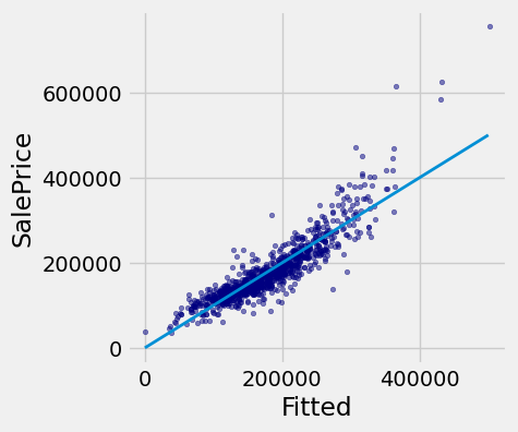
If the predictions were perfect, then a scatter plot of the predicted and actual values would be a straight line with slope 1. We see that most dots fall near that line, but there is some error in the predictions.

def fit(row):
    return sum(best_slopes * np.array(row))

test['Fitted'] = test_attributes.apply(fit, axis=1)

fig, ax = plt.subplots(figsize=(4,4))

ax.scatter(
    test['Fitted'], 
    test['SalePrice'],   
    color='navy', 
    alpha=0.5,
    s=10
)

x_label = 'Fitted'
y_label = 'SalePrice'

plt.ylabel(y_label)
plt.xlabel(x_label)

plt.plot([0, 5e5], [0, 5e5], lw=2)

plt.show()

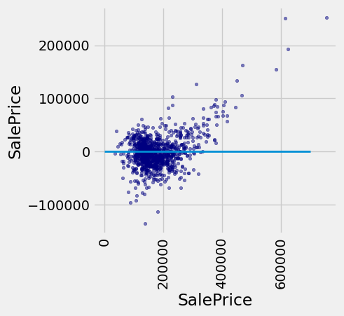
A residual plot for multiple regression typically compares the errors (residuals) to the actual values of the predicted variable. We see in the residual plot below that we have systematically underestimated the value of expensive houses, shown by the many positive residual values on the right side of the graph.

test['Residual'] = test_prices-test_attributes.apply(fit, axis=1)

fig, ax = plt.subplots(figsize=(4,4))

ax.scatter(
    test['SalePrice'], 
    test['Residual'],   
    color='navy', 
    alpha=0.5,
    s=10
)

x_label = 'SalePrice'

y_label = 'SalePrice'

plt.ylabel(y_label)

plt.xlabel(x_label)

plt.xticks(rotation=90)

plt.plot([0, 7e5], [0, 0], lw=2)

plt.show()

As with simple linear regression, interpreting the result of a predictor is at least as important as making predictions. There are many lessons about interpreting multiple regression that are not included in this textbook. A natural next step after completing this text would be to study linear modeling and regression in further depth.

20.6.3. Nearest Neighbors for Regression

Another approach to predicting the sale price of a house is to use the price of similar houses. This nearest neighbor approach is very similar to our classifier. To speed up computation, we will only use the attributes that had the highest correlation with the sale price in our original analysis.

train_nn = train.iloc[:, [0, 1, 2, 3, 4, 8]]
test_nn = test.iloc[:, [0, 1, 2, 3, 4, 8]]
train_nn

	SalePrice	1st Flr SF	2nd Flr SF	Total Bsmt SF	Garage Area	Year Built
2142	127000	864	0	864.0	576.0	1972
2201	148500	567	531	531.0	216.0	1930
2643	110000	813	0	813.0	270.0	1930
1703	317000	1143	1330	1143.0	852.0	2004
26	126000	882	0	882.0	525.0	1970
...	...	...	...	...	...	...
867	198500	840	885	840.0	550.0	2002
1396	152400	864	486	576.0	627.0	1941
1222	87000	453	453	348.0	231.0	1937
691	115000	818	406	818.0	210.0	1926
2149	200000	860	869	860.0	542.0	2002

1001 rows × 6 columns

The computation of closest neighbors is identical to a nearest-neighbor classifier. In this case, we will exclude the 'SalePrice' rather than the 'Class' column from the distance computation. The five nearest neighbors of the first test row are shown below.

def distance(pt1, pt2):
    """The distance between two points, represented as arrays."""
    return np.sqrt(np.sum((pt1 - pt2) ** 2))
    
def row_distance(row1, row2):
    """The distance between two rows of a table."""
    return distance(np.array(row1), np.array(row2))

def distances(training, example, output):
    """Compute the distance from example for each row in training."""
    dists = []
    attributes = training.drop(columns=[output])
    for row in range(len(attributes)):
        dists.append(row_distance(attributes.iloc[row], example))
    training['Distance'] = dists
    #print(training)
    return training

def closest(training, example, k, output):
    """Return a table of the k closest neighbors to example."""
    distance = distances(training, example, output).sort_values(by=['Distance']).take(np.arange(k))
    return distance

train_nn_A = train_nn.copy()
example_nn_row = test_nn.drop(test_nn.columns[0], axis=1).iloc[0]
closest(train_nn_A, example_nn_row, 5, 'SalePrice')

	SalePrice	1st Flr SF	2nd Flr SF	Total Bsmt SF	Garage Area	Year Built	Distance
141	165500	1700	0	1398.0	447.0	1959	72.270326
375	200000	1671	0	1427.0	484.0	1978	112.058021
578	150000	1620	0	1281.0	490.0	1976	117.209215
2715	180000	1721	0	1461.0	440.0	1968	132.653684
1183	290000	1671	0	1426.0	550.0	1976	138.859641

One simple method for predicting the price is to average the prices of the nearest neighbors.

example_nn_row

1st Flr SF       1721.0
2nd Flr SF          0.0
Total Bsmt SF    1331.0
Garage Area       464.0
Year Built       1957.0
Name: 1924, dtype: float64

def predict_nn(example):
    """Return the majority class among the k nearest neighbors."""
    train_nn_B = train_nn.copy()
    
    col_sales_price = closest(train_nn_B, example, 5, 'SalePrice')
    return np.average(col_sales_price['SalePrice'])

predict_nn(example_nn_row)

np.float64(197100.0)

Finally, we can inspect whether our prediction is close to the true sale price for our one test example. Looks reasonable!

print('Actual sale price:', test_nn['SalePrice'].iloc[0])
print('Predicted sale price using nearest neighbors:', predict_nn(example_nn_row))

Actual sale price: 174850
Predicted sale price using nearest neighbors: 197100.0

20.6.3.1. Evaluation

To evaluate the performance of this approach for the whole test set, we apply predict_nn to each test example, then compute the root mean squared error of the predictions. Computation of the predictions may take several minutes.

def predict_nn(example):
    """Return the majority class among the k nearest neighbors."""
    train_nn_B = train_nn.copy()
    
    col_sales_price = closest(train_nn_B, example, 5, 'SalePrice')
    return np.average(col_sales_price['SalePrice']).item(0)

predict_nn(example_nn_row)

197100.0

test_nn_C = test_nn.copy()
test_nn_drop = test_nn_C.drop(columns=['SalePrice'])

nn_test_predictions = test_nn_drop.apply(predict_nn, axis=1)
rmse_nn = np.mean((test_prices - nn_test_predictions) ** 2) ** 0.5

print('Test set RMSE for multiple linear regression: ', rmse_linear)
print('Test set RMSE for nearest neighbor regression:', rmse_nn)

Test set RMSE for multiple linear regression:  30125.47384508643
Test set RMSE for nearest neighbor regression: 33266.600357451876

For these data, the errors of the two techniques are quite similar! For different data sets, one technique might outperform another. By computing the RMSE of both techniques on the same data, we can compare methods fairly. One note of caution: the difference in performance might not be due to the technique at all; it might be due to the random variation due to sampling the training and test sets in the first place.

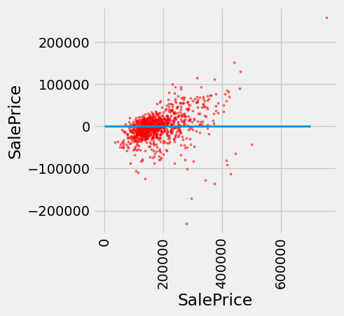
Finally, we can draw a residual plot for these predictions. We still underestimate the prices of the most expensive houses, but the bias does not appear to be as systematic. However, fewer residuals are very close to zero, indicating that fewer prices were predicted with very high accuracy.

test['Residual'] = test_prices-nn_test_predictions

fig, ax = plt.subplots(figsize=(4,4))

ax.scatter(
    test['SalePrice'], 
    test['Residual'],   
    color='red', 
    alpha=0.5,
    s=5
)

x_label = 'SalePrice'
y_label = 'SalePrice'
plt.ylabel(y_label)
plt.xlabel(x_label)
plt.xticks(rotation=90)
plt.plot([0, 7e5], [0, 0], lw=2)
plt.show()