19.1. Linear Regression with Python#
Your neighbor is a real estate agent and wants some help predicting housing prices for regions in the USA. It would be great if you could somehow create a model for her that allows her to put in a few features of a house and returns back an estimate of what the house would sell for.
She has asked you if you could help her out with your new data science skills. You say yes, and decide that Linear Regression might be a good path to solve this problem!
Your neighbor then gives you some information about a bunch of houses in regions of the United States,it is all in the data set: USA_Housing.csv.
The data contains the following columns:
‘Avg. Area Income’: Avg. Income of residents of the city house is located in.
‘Avg. Area House Age’: Avg Age of Houses in same city
‘Avg. Area Number of Rooms’: Avg Number of Rooms for Houses in same city
‘Avg. Area Number of Bedrooms’: Avg Number of Bedrooms for Houses in same city
‘Area Population’: Population of city house is located in
‘Price’: Price that the house sold at
‘Address’: Address for the house
We’ve been able to get some data from your neighbor for housing prices as a csv set, let’s get our environment ready with the libraries we’ll need and then import the data.
path_data='../../data/'
import pandas as pd
import numpy as np
# %pip install scikit-learn --quiet
import sklearn
import matplotlib.pyplot as plt
import seaborn as sns
%matplotlib inline
USAhousing = pd.read_csv(path_data + 'USA_Housing.csv')
USAhousing.head()
| Avg. Area Income | Avg. Area House Age | Avg. Area Number of Rooms | Avg. Area Number of Bedrooms | Area Population | Price | Address | |
|---|---|---|---|---|---|---|---|
| 0 | 79545.458574 | 5.682861 | 7.009188 | 4.09 | 23086.800503 | 1.059034e+06 | 208 Michael Ferry Apt. 674\nLaurabury, NE 3701... |
| 1 | 79248.642455 | 6.002900 | 6.730821 | 3.09 | 40173.072174 | 1.505891e+06 | 188 Johnson Views Suite 079\nLake Kathleen, CA... |
| 2 | 61287.067179 | 5.865890 | 8.512727 | 5.13 | 36882.159400 | 1.058988e+06 | 9127 Elizabeth Stravenue\nDanieltown, WI 06482... |
| 3 | 63345.240046 | 7.188236 | 5.586729 | 3.26 | 34310.242831 | 1.260617e+06 | USS Barnett\nFPO AP 44820 |
| 4 | 59982.197226 | 5.040555 | 7.839388 | 4.23 | 26354.109472 | 6.309435e+05 | USNS Raymond\nFPO AE 09386 |
USAhousing.info()
<class 'pandas.core.frame.DataFrame'>
RangeIndex: 5000 entries, 0 to 4999
Data columns (total 7 columns):
 #   Column                        Non-Null Count  Dtype
---  ------                        --------------  -----
 0   Avg. Area Income              5000 non-null   float64
 1   Avg. Area House Age           5000 non-null   float64
 2   Avg. Area Number of Rooms     5000 non-null   float64
 3   Avg. Area Number of Bedrooms  5000 non-null   float64
 4   Area Population               5000 non-null   float64
 5   Price                         5000 non-null   float64
 6   Address                       5000 non-null   object
dtypes: float64(6), object(1)
memory usage: 273.6+ KB
USAhousing.describe()
| Avg. Area Income | Avg. Area House Age | Avg. Area Number of Rooms | Avg. Area Number of Bedrooms | Area Population | Price | |
|---|---|---|---|---|---|---|
| count | 5000.000000 | 5000.000000 | 5000.000000 | 5000.000000 | 5000.000000 | 5.000000e+03 |
| mean | 68583.108984 | 5.977222 | 6.987792 | 3.981330 | 36163.516039 | 1.232073e+06 |
| std | 10657.991214 | 0.991456 | 1.005833 | 1.234137 | 9925.650114 | 3.531176e+05 |
| min | 17796.631190 | 2.644304 | 3.236194 | 2.000000 | 172.610686 | 1.593866e+04 |
| 25% | 61480.562388 | 5.322283 | 6.299250 | 3.140000 | 29403.928702 | 9.975771e+05 |
| 50% | 68804.286404 | 5.970429 | 7.002902 | 4.050000 | 36199.406689 | 1.232669e+06 |
| 75% | 75783.338666 | 6.650808 | 7.665871 | 4.490000 | 42861.290769 | 1.471210e+06 |
| max | 107701.748378 | 9.519088 | 10.759588 | 6.500000 | 69621.713378 | 2.469066e+06 |
USAhousing.columns
Index(['Avg. Area Income', 'Avg. Area House Age', 'Avg. Area Number of Rooms',
       'Avg. Area Number of Bedrooms', 'Area Population', 'Price', 'Address'],
      dtype='object')
19.1.1. Exploratory Data Analysis#
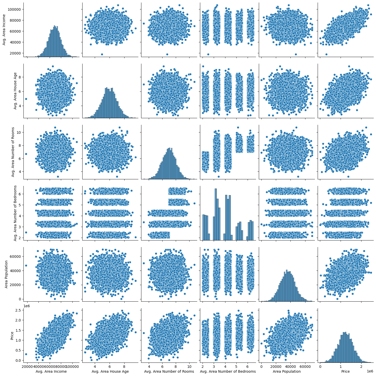
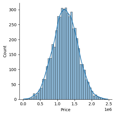
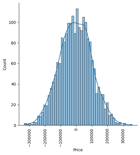
Let’s create some simple plots to check out the data!
sns.pairplot(USAhousing)
<seaborn.axisgrid.PairGrid at 0x11472d7f0>
sns.displot(USAhousing['Price'], kde=True, height=4)
<seaborn.axisgrid.FacetGrid at 0x1148e9a90>
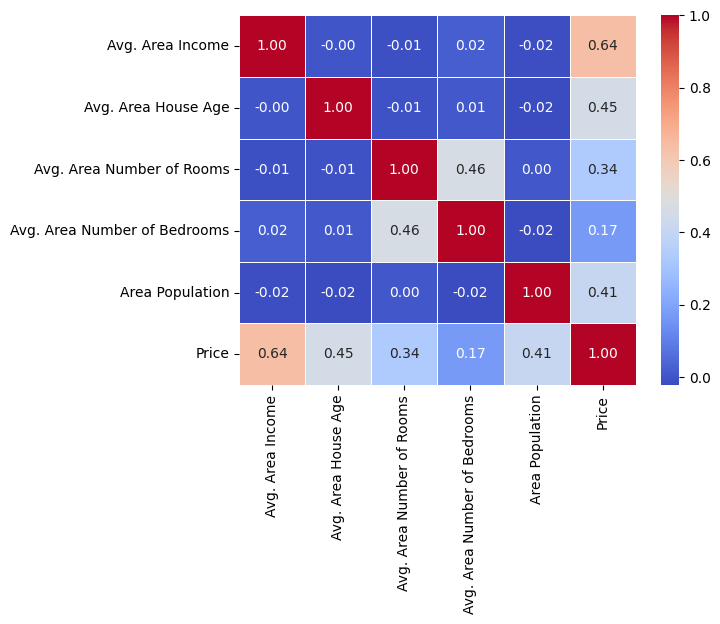
# sns.heatmap(USAhousing.drop('Address', axis=1).corr(), annot=True, cmap='viridis', fmt=".2f", linewidths=.5)
sns.heatmap(USAhousing.drop('Address', axis=1).corr(), annot=True, cmap='coolwarm', fmt=".2f", linewidths=.5)
<Axes: >
19.1.2. Training a Linear Regression Model#
Let’s now begin to train out regression model! We will need to first split up our data into an X array that contains the features to train on, and a y array with the target variable, in this case the Price column. We will toss out the Address column because it only has text info that the linear regression model can’t use.
19.1.2.1. X and y arrays#
X = USAhousing[['Avg. Area Income', 'Avg. Area House Age', 'Avg. Area Number of Rooms',
               'Avg. Area Number of Bedrooms', 'Area Population']]
y = USAhousing['Price']
19.1.3. Train Test Split#
Now let’s split the data into a training set and a testing set. We will train out model on the training set and then use the test set to evaluate the model.
from sklearn.model_selection import train_test_split
X_train, X_test, y_train, y_test = train_test_split(X, y, test_size=0.4, random_state=101)
19.1.4. Creating and Training the Model#
from sklearn.linear_model import LinearRegression
lm = LinearRegression()
lm.fit(X_train,y_train)
LinearRegression()In a Jupyter environment, please rerun this cell to show the HTML representation or trust the notebook.
On GitHub, the HTML representation is unable to render, please try loading this page with nbviewer.org.
Parameters
| fit_intercept | True | |
| copy_X | True | |
| tol | 1e-06 | |
| n_jobs | None | |
| positive | False |
19.1.5. Model Evaluation#
Let’s evaluate the model by checking out it’s coefficients and how we can interpret them.
### print the intercept

print(lm.intercept_)
-2640159.7968517053
coeff_df = pd.DataFrame(lm.coef_,X.columns,columns=['Coefficient'])
coeff_df
| Coefficient | |
|---|---|
| Avg. Area Income | 21.528276 |
| Avg. Area House Age | 164883.282027 |
| Avg. Area Number of Rooms | 122368.678027 |
| Avg. Area Number of Bedrooms | 2233.801864 |
| Area Population | 15.150420 |
Interpreting the coefficients:
Holding all other features fixed, a 1 unit increase in Avg. Area Income is associated with an **increase of $21.52 **.
Holding all other features fixed, a 1 unit increase in Avg. Area House Age is associated with an **increase of $164883.28 **.
Holding all other features fixed, a 1 unit increase in Avg. Area Number of Rooms is associated with an **increase of $122368.67 **.
Holding all other features fixed, a 1 unit increase in Avg. Area Number of Bedrooms is associated with an **increase of $2233.80 **.
Holding all other features fixed, a 1 unit increase in Area Population is associated with an **increase of $15.15 **.
Does this make sense? Probably not because I made up this data. If you want real data to repeat this sort of analysis, check out the boston dataset :
from sklearn.datasets import load_boston
boston = load_boston()
print(boston.DESCR)
boston_df = boston.data
19.1.6. Predictions from our Model#
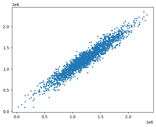
Let’s grab predictions off our test set and see how well it did!
predictions = lm.predict(X_test)
plt.scatter(y_test,predictions, s=5)
<matplotlib.collections.PathCollection at 0x11775ed50>
Residual Histogram
sns.displot((y_test-predictions), bins=50, kde=True)
plt.xticks(rotation=90)
plt.show()
19.1.7. Regression Evaluation Metrics#
Here are three common evaluation metrics for regression problems:
Mean Absolute Error (MAE) is the mean of the absolute value of the errors:
Mean Squared Error (MSE) is the mean of the squared errors:
Root Mean Squared Error (RMSE) is the square root of the mean of the squared errors:
Comparing these metrics:
MAE is the easiest to understand, because it’s the average error.
MSE is more popular than MAE, because MSE “punishes” larger errors, which tends to be useful in the real world.
RMSE is even more popular than MSE, because RMSE is interpretable in the “y” units.
All of these are loss functions, because we want to minimize them.
from sklearn import metrics
print('MAE:', metrics.mean_absolute_error(y_test, predictions))
print('MSE:', metrics.mean_squared_error(y_test, predictions))
print('RMSE:', np.sqrt(metrics.mean_squared_error(y_test, predictions)))
MAE: 82288.22251914947
MSE: 10460958907.2096
RMSE: 102278.82922291201
This was your first real Machine Learning experience! Congrats on helping your neighbor out! We’ll let this end here for now, but go ahead and explore the Boston Dataset mentioned earlier if this particular data set was interesting to you!