14. Descriptive Statistics & Distribution#
Goals
Describe a variable using center, spread, and shape
Compute descriptive statistics: mean, median, variance, standard deviation
Understand distributions
Connect probability to data-generating processes
Randomness
The Law of Large Numbers
### headers
import numpy as np
import pandas as pd
import matplotlib.pyplot as plt
import seaborn as sns
14.1. Data and Variables#
When describing data, make sure you cover center, spread, and shape.
tips = sns.load_dataset('tips')
tips                      ### size means number of ppl in the party
| total_bill | tip | sex | smoker | day | time | size | |
|---|---|---|---|---|---|---|---|
| 0 | 16.99 | 1.01 | Female | No | Sun | Dinner | 2 |
| 1 | 10.34 | 1.66 | Male | No | Sun | Dinner | 3 |
| 2 | 21.01 | 3.50 | Male | No | Sun | Dinner | 3 |
| 3 | 23.68 | 3.31 | Male | No | Sun | Dinner | 2 |
| 4 | 24.59 | 3.61 | Female | No | Sun | Dinner | 4 |
| ... | ... | ... | ... | ... | ... | ... | ... |
| 239 | 29.03 | 5.92 | Male | No | Sat | Dinner | 3 |
| 240 | 27.18 | 2.00 | Female | Yes | Sat | Dinner | 2 |
| 241 | 22.67 | 2.00 | Male | Yes | Sat | Dinner | 2 |
| 242 | 17.82 | 1.75 | Male | No | Sat | Dinner | 2 |
| 243 | 18.78 | 3.00 | Female | No | Thur | Dinner | 2 |
244 rows × 7 columns
tips.shape ### a dataframe has shape, which is a tuple
(244, 7)
14.1.1. Population vs sample#
Population is the full group we care about (e.g., “all lunch bills at the restaurant this year”), whereas sample is the subset we actually measured (e.g., the 244 rows in the tips dataset). We only ever see the sample, but we talk like we know the population.
14.1.2. Variable vs Observation#
Each row in the dataframe/dataset is an observation (e.g., one restaurant bill), whereas columns are variables (e.g., total_bill, tip, smoker, time (Dinner/Lunch), etc.).
Quantitative variable: e.g., total_bill (numeric, measured)
Categorical variable: time (Lunch vs Dinner), smoker (Yes/No)
14.1.3. Distribution#
A distribution shows how often different values occur. For numeric data:
Are most bills around $10? $20? $50?
Are there a few very large bills? (outliers)
For categorical data:
How common is “Dinner” vs “Lunch”?
14.1.4. Descriptive Statistics#
df.describe() gives you the descriptive statistics of the dataset.
tips.describe()
| total_bill | tip | size | |
|---|---|---|---|
| count | 244.000000 | 244.000000 | 244.000000 |
| mean | 19.785943 | 2.998279 | 2.569672 |
| std | 8.902412 | 1.383638 | 0.951100 |
| min | 3.070000 | 1.000000 | 1.000000 |
| 25% | 13.347500 | 2.000000 | 2.000000 |
| 50% | 17.795000 | 2.900000 | 2.000000 |
| 75% | 24.127500 | 3.562500 | 3.000000 |
| max | 50.810000 | 10.000000 | 6.000000 |
Key summaries for a numeric variable:
Mean (average)
Median (middle value)
Standard deviation (typical distance from the mean)
IQR (middle 50% range)
Let’s compute them for total_bill.
14.1.5. Center: mean vs median#
col = tips['total_bill']

summary = pd.DataFrame({
    'mean': [col.mean()],
    'median': [col.median()],
    'std (SD)': [col.std()],
    'IQR': [col.quantile(0.75) - col.quantile(0.25)]
})
summary
| mean | median | std (SD) | IQR | |
|---|---|---|---|---|
| 0 | 19.785943 | 17.795 | 8.902412 | 10.78 |
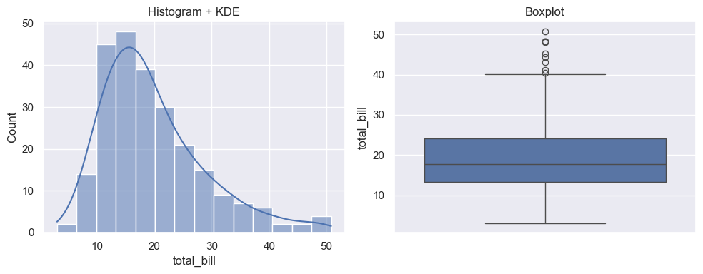
14.1.6. Visualizing One Variable#
We’ll use:
Histogram (counts or density)
Boxplot (median, quartiles, outliers)
KDE / density curve (smoothed shape)
Interpretation checklist: center / spread / shape / outliers.
sns.set_theme()

fig, axes = plt.subplots(1, 2, figsize=(10,4))

sns.histplot(tips, x='total_bill', kde=True, ax=axes[0])
axes[0].set_title('Histogram + KDE')

sns.boxplot(y=tips['total_bill'], ax=axes[1])
axes[1].set_title('Boxplot')

plt.tight_layout()
14.2. Distributions#
14.2.1. Normal Distribution#
A normal distribution—also called a Gaussian distribution—is a symmetrical, bell-shaped probability distribution centered on the mean, where most data points cluster around that mean with frequencies tapering off equally toward both extremes.
Key Properties:
Defined by its mean (μ) and standard deviation (σ).
The
mean,median, andmodeare equal and located at the center.Symmetrical: the left and right sides are mirror images.
68% of data falls within 1 standard deviation, 95% within 2, and 99.7% within 3 standard deviations from the mean (“Empirical Rule”).
Frequently models real-world phenomena due to the Central Limit Theorem.
Example Applications:
Heights of People: Human heights in a given population typically follow a normal distribution—most people are near the average height, with fewer extremely short or tall.
IQ Scores: Measured intelligence is designed to follow a normal curve, with an average of 100 and most people close to the average.
Measurement Errors: Repeated measurements of something (e.g., lengths, weights) often cluster around the true value, following a normal distribution.
Test Scores: Large-scale standardized test results (e.g., SAT, GRE) often approximate a normal distribution after some normalization.
Example |
Mean (μ) |
Standard Deviation (σ) |
What is Measured |
|---|---|---|---|
Adult heights |
170 cm |
10 cm |
Human height distribution |
IQ scores |
100 |
15 |
Intelligence |
SAT scores |
1050 |
200 |
Standardized tests |
Let us use the random module in NumPy to explore.
from numpy import random
random.seed(42)

x = random.normal(size=(2, 3))
print(type(x))
print(x)
<class 'numpy.ndarray'>
[[ 0.49671415 -0.1382643   0.64768854]
 [ 1.52302986 -0.23415337 -0.23413696]]
Now let’s add mean and standard deviation (because this is a normal distribution). Here we are controlling the center and the spread of the distribution.
### generate a random normal distribution of size 2X3 with mean at 1 and SD of 2

random.seed(42)
x = random.normal(loc=1, scale=2, size=(2, 3))
print(x)
[[1.99342831 0.7234714  2.29537708]
 [4.04605971 0.53169325 0.53172609]]
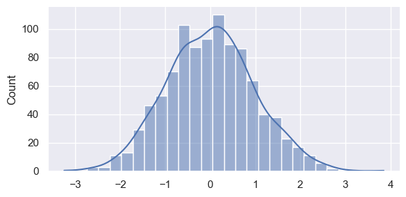
Time for some visualization. Note that we are using height and aspect (ratio) to control figure size.
random.seed(42)
np.random.seed(42)
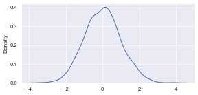
sns.displot(random.normal(size=1000), height=3, aspect=2,kde=True)
<seaborn.axisgrid.FacetGrid at 0x1159eec10>
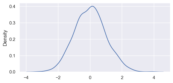
A KDE only plot. Note that we are controlling figure size by
plt.figure(figsize)dpi
random.seed(42)

np.random.seed(42)

plt.figure(figsize=(6.5, 3))
sns.kdeplot(random.normal(size=1000))
<Axes: ylabel='Density'>
Now let’s add dpi to control figure size.
np.random.seed(42)

import matplotlib as mpl
with mpl.rc_context({"figure.dpi": 100}):
    plt.figure(figsize=(6.5, 3))
    sns.kdeplot(random.normal(size=1000))
np.random.seed(42)

import matplotlib as mpl
with mpl.rc_context({"figure.dpi": 50}):
    plt.figure(figsize=(6.5, 3))
    sns.kdeplot(random.normal(size=1000))
14.2.2. Binomial Distribution#
A binomial distribution is a discrete probability distribution that models the number of successes in a fixed number of independent trials, where each trial has only two outcomes: “success” or “failure.” Every trial must have the same probability of success. This distribution is fundamental for analyzing repeated yes/no-type experiments (Bernoulli trials) and appears frequently in statistics and data science.
Key Features:
There are
nfixed trials.Each trial is independent.
There are only two possible outcomes per trial (success or failure).
The chance of success
pis constant for each trial.
For example, flipping a fair coin 10 times and counting the number of heads. Here, each flip is independent, and the probability of heads (success) is 0.5. The distribution of the number of heads follows a binomial distribution with n=10, p=0.5.
# binomial vs normal distributions
random.seed(42)

norm = random.normal(loc=50, scale=5, size=1000)
bino = random.binomial(n=100, p=0.5, size=1000)
fig, ax = plt.subplots(figsize=(4, 3))
sns.kdeplot(data=norm, label='Normal', color='red')
sns.kdeplot(data=bino, label='Binomial', color='green')
plt.tight_layout()
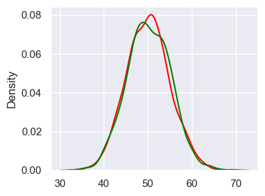
Visually comparing normal distribution and binomial distribution.
### test out 1 scaler
random.binomial(n=100, p=0.5, size=1)
array([45])
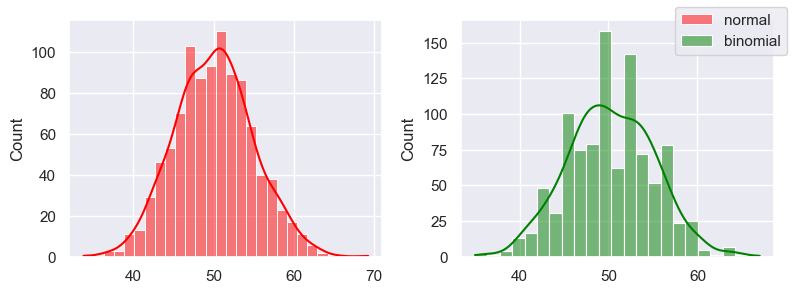
### normal distribution vs binomial
### binomial approximates normal distribution when n is big (np >=5)
### binomial "spikes" because it's integers

random.seed(42)
norm = random.normal(loc=50, scale=5, size=1000)  ### mean=50, SD=5 to match binomial
bino = random.binomial(n=100, p=0.5, size=1000)

fig, ax = plt.subplots(1, 2, figsize=(8, 3))
sns.histplot(norm, label='normal', color='red', ax=ax[0], kde=True)
sns.histplot(bino, label="binomial", color='green', ax=ax[1], kde=True)
fig.legend()
fig.tight_layout()
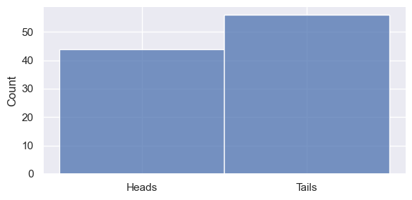
Coin flipping! (If you count the numbers of heads, it will be a normal distribution)
# Define the coin sides
coin = ['Heads', 'Tails']

# Simulate 100 coin flips
random.seed(42)
flips = np.random.choice(coin, size=100)

# Count the number of heads
num_heads = np.count_nonzero(flips == 'Heads')

print("Number of Heads:", num_heads)

sns.displot(flips, height=3, aspect=2, bins=10, kde=False)
Number of Heads: 44
<seaborn.axisgrid.FacetGrid at 0x11598d1d0>
14.2.3. Uniform Distribution#
A uniform distribution is a probability distribution where every outcome within a certain range is equally likely to occur. This means there is no bias—each result has the same probability as any other within the specified set.
Examples:
Rolling a fair six-sided die. Each face (1 through 6) has a 1/6 chance of appearing, so the probability of rolling any particular number is equal.
Flipping a fair coin. Heads and tails each have a 50% chance.
The numpy.random.uniform() method draws samples from a uniform distribution. Samples are uniformly distributed over the half-open interval [low, high) (includes low, but excludes high). In other words, any value within the given interval is equally likely to be drawn by uniform.
The syntax:
random.uniform(low=0.0, high=1.0, size=None)
random.seed(42)

unif1 = random.uniform()                               ### return 1 number [0, 1)
unif2 = random.uniform(low=1, high=5, size=3)          ### return size=3 numbers [0, 1)
unif3 = random.uniform(low=5, high=10, size=(3, 3))    ### return a 3x3 2D array
unif4 = np.round(random.uniform(low=5, high=10, size=(3, 3)), 2)     ### rounded
unif5 = random.randint(low=5, high=10, size=(3, 3))    ### int

for unif in [ unif1, unif2, unif3, unif4, unif5 ]:
    print(unif, '\n')
0.3745401188473625

[4.80285723 3.92797577 3.39463394]

[[5.7800932  5.7799726  5.29041806]
 [9.33088073 8.00557506 8.54036289]
 [5.10292247 9.84954926 9.1622132 ]]

[[6.06 5.91 5.92]
 [6.52 7.62 7.16]
 [6.46 8.06 5.7 ]]

[[8 8 7]
 [8 8 5]
 [7 9 7]]
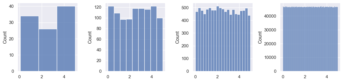
14.2.3.1. Best Example: Rolling Die#
We eventually flip 1 million times here and see that all 6 numbers and have equal probability distribution.
### flip for many times

fig, axes = plt.subplots(1, 5, figsize=(12, 3))

flips = []
for i, ran in enumerate([ 10, 100, 1000, 10000, 1000000 ]):
    for flip in range(ran):                  ### if n > 26, print vertically
        flips.append(random.randint(1, 7))
    # sns.histplot(flips, ax=axes[i])
    sns.histplot(flips, ax=axes[i], bins=6)

plt.tight_layout()
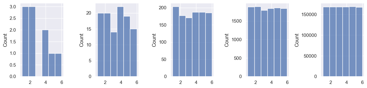
Note that binning can affect the plotting greatly.
### displot with height and aspect

sns.displot(flips, height=2.5, aspect=3/2)
sns.displot(flips, height=2.5, aspect=3/2, bins=6)
<seaborn.axisgrid.FacetGrid at 0x1169302d0>
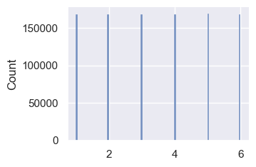
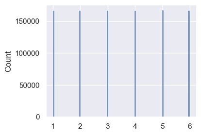
Now use randint() to append 1000,000 random ints.
### flip for 1 million times
random.seed(42)

flips2 = []
for flip in range(1000000):
    flips2.append(random.randint(1, 7))

plt.figure(figsize=(4, 3))
sns.histplot(flips2)

print(len(flips2))
print(len(flips2)/6)
1000000
166666.66666666666
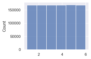
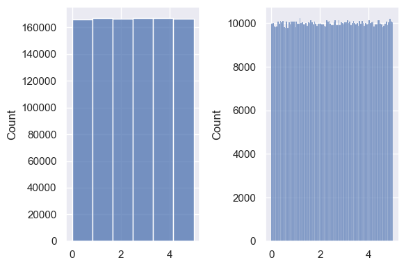
Use the random.uniform() function to check. Looks uniform to me.
random.seed(42)
unif = random.uniform(0, 5, size=1000000)

fig, ax = plt.subplots(1, 2, figsize=(6, 4))

sns.histplot(data=unif, bins=6, ax=ax[0])
sns.histplot(data=unif, bins=100, ax=ax[1])

plt.tight_layout()
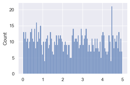
But, when we have smaller n and larger bins, we see spikes:
random.seed(42)
unif = random.uniform(0, 5, size=1000)    ### low, high exclusive
sns.displot(data=unif, kind='hist', height=3, aspect=3/2, bins=100)
# sns.displot(unif, kind='kde')
# plt.show()
<seaborn.axisgrid.FacetGrid at 0x119279f90>
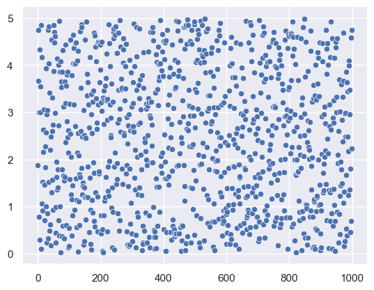
Using scatter plot to visualize.
random.seed(42)
unif = random.uniform(0, 5, size=1000)

sns.scatterplot(data=unif)
<Axes: >
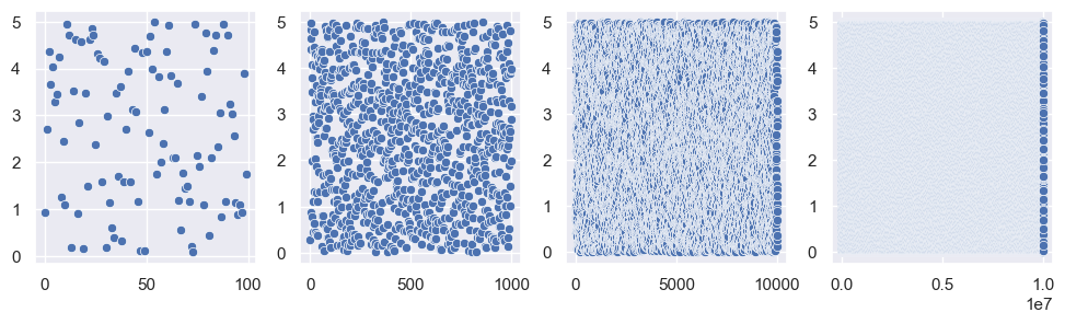
fig, axes = plt.subplots(1, 4, figsize=(12, 3)) ### now we have one fig with two axes

unif1 = random.uniform(0, 5, size=100)
unif2 = random.uniform(0, 5, size=1000)
unif3 = random.uniform(0, 5, size=10000)
unif4 = random.uniform(0, 5, size=10000000)

sns.scatterplot(unif1, ax=axes[0])
sns.scatterplot(unif2, ax=axes[1])
sns.scatterplot(unif3, ax=axes[2])
sns.scatterplot(unif4, ax=axes[3])
<Axes: >
Now, produce a similar plot like the one above for random.randn(). Note the binning strategy here.
fig, axes = plt.subplots(1, 4, figsize=(12, 3)) ### now we have one fig with two axes

datasets = [ unif1, unif2, unif3, unif4 ]
for i, data in enumerate(datasets):

    q25, q75 = np.percentile(data, [25, 75])            ### bins
    bin_width = 2 * (q75 - q25) * len(data) ** (-1/3)   ### bins
    bins = int((data.max() - data.min()) / bin_width)   ### bins

    sns.histplot(data=data, ax=axes[i], bins=bins)      ### plot

plt.tight_layout()
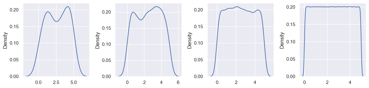
Visualizing using KDE.
fig, axes = plt.subplots(1, 4, figsize=(12, 3)) ### now we have one fig with two axes

for i, data in enumerate(datasets):

    ### bins ###
    q25, q75 = np.percentile(data, [25, 75])
    bin_width = 2 * (q75 - q25) * len(data) ** (-1/3)
    bins = int((data.max() - data.min()) / bin_width)   ### bins #

    sns.kdeplot(data=data, ax=axes[i])      ### plot

plt.tight_layout()
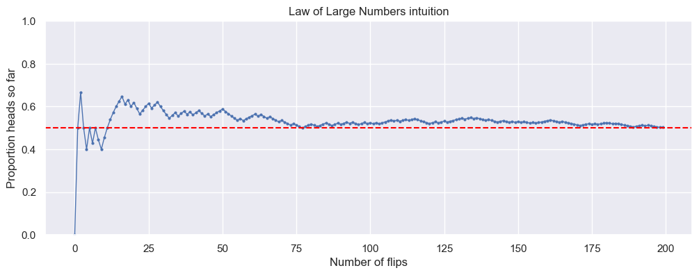
14.3. The Law of Large Numbers#
We’ll simulate coin flips to show:
Randomness
Law of large numbers (the running average stabilizes)
Each flip is 0 (tails) or 1 (heads).
tips.sample(5)
| total_bill | tip | sex | smoker | day | time | size | |
|---|---|---|---|---|---|---|---|
| 101 | 15.38 | 3.00 | Female | Yes | Fri | Dinner | 2 |
| 127 | 14.52 | 2.00 | Female | No | Thur | Lunch | 2 |
| 75 | 10.51 | 1.25 | Male | No | Sat | Dinner | 2 |
| 22 | 15.77 | 2.23 | Female | No | Sat | Dinner | 2 |
| 220 | 12.16 | 2.20 | Male | Yes | Fri | Lunch | 2 |
rng = np.random.default_rng(42)

type(rng.integers(0, 2, 10))
rng = np.random.default_rng(42)
flips = rng.integers(0, 2, 200)
flips
array([0, 1, 1, 0, 0, 1, 0, 1, 0, 0, 1, 1, 1, 1, 1, 1, 1, 0, 1, 0, 1, 0,
       0, 1, 1, 1, 0, 1, 1, 0, 0, 0, 0, 1, 1, 0, 1, 1, 0, 1, 0, 1, 1, 0,
       0, 1, 0, 1, 1, 1, 1, 0, 0, 0, 0, 0, 1, 0, 1, 1, 1, 1, 0, 1, 0, 0,
       1, 0, 0, 0, 1, 0, 0, 0, 1, 0, 0, 0, 1, 1, 1, 0, 0, 1, 1, 1, 0, 0,
       1, 1, 0, 1, 1, 0, 1, 0, 0, 1, 1, 0, 1, 0, 1, 0, 1, 1, 1, 1, 0, 1,
       0, 1, 1, 0, 1, 1, 0, 0, 0, 0, 0, 1, 1, 0, 1, 1, 0, 1, 1, 1, 1, 1,
       0, 1, 1, 0, 1, 0, 0, 0, 1, 0, 0, 0, 1, 1, 0, 0, 1, 0, 1, 0, 1, 0,
       0, 1, 0, 1, 1, 1, 1, 1, 0, 0, 0, 1, 0, 0, 0, 0, 0, 0, 1, 1, 1, 0,
       1, 0, 1, 1, 1, 0, 0, 1, 0, 0, 0, 0, 0, 0, 1, 1, 1, 0, 1, 0, 0, 0,
       0, 1])
np.arange(len(flips)) + 1 ### fixed and grow linearly
array([  1,   2,   3,   4,   5,   6,   7,   8,   9,  10,  11,  12,  13,
        14,  15,  16,  17,  18,  19,  20,  21,  22,  23,  24,  25,  26,
        27,  28,  29,  30,  31,  32,  33,  34,  35,  36,  37,  38,  39,
        40,  41,  42,  43,  44,  45,  46,  47,  48,  49,  50,  51,  52,
        53,  54,  55,  56,  57,  58,  59,  60,  61,  62,  63,  64,  65,
        66,  67,  68,  69,  70,  71,  72,  73,  74,  75,  76,  77,  78,
        79,  80,  81,  82,  83,  84,  85,  86,  87,  88,  89,  90,  91,
        92,  93,  94,  95,  96,  97,  98,  99, 100, 101, 102, 103, 104,
       105, 106, 107, 108, 109, 110, 111, 112, 113, 114, 115, 116, 117,
       118, 119, 120, 121, 122, 123, 124, 125, 126, 127, 128, 129, 130,
       131, 132, 133, 134, 135, 136, 137, 138, 139, 140, 141, 142, 143,
       144, 145, 146, 147, 148, 149, 150, 151, 152, 153, 154, 155, 156,
       157, 158, 159, 160, 161, 162, 163, 164, 165, 166, 167, 168, 169,
       170, 171, 172, 173, 174, 175, 176, 177, 178, 179, 180, 181, 182,
       183, 184, 185, 186, 187, 188, 189, 190, 191, 192, 193, 194, 195,
       196, 197, 198, 199, 200])
flips.cumsum() ### grow slower because of 0, 1
array([  0,   1,   2,   2,   2,   3,   3,   4,   4,   4,   5,   6,   7,
         8,   9,  10,  11,  11,  12,  12,  13,  13,  13,  14,  15,  16,
        16,  17,  18,  18,  18,  18,  18,  19,  20,  20,  21,  22,  22,
        23,  23,  24,  25,  25,  25,  26,  26,  27,  28,  29,  30,  30,
        30,  30,  30,  30,  31,  31,  32,  33,  34,  35,  35,  36,  36,
        36,  37,  37,  37,  37,  38,  38,  38,  38,  39,  39,  39,  39,
        40,  41,  42,  42,  42,  43,  44,  45,  45,  45,  46,  47,  47,
        48,  49,  49,  50,  50,  50,  51,  52,  52,  53,  53,  54,  54,
        55,  56,  57,  58,  58,  59,  59,  60,  61,  61,  62,  63,  63,
        63,  63,  63,  63,  64,  65,  65,  66,  67,  67,  68,  69,  70,
        71,  72,  72,  73,  74,  74,  75,  75,  75,  75,  76,  76,  76,
        76,  77,  78,  78,  78,  79,  79,  80,  80,  81,  81,  81,  82,
        82,  83,  84,  85,  86,  87,  87,  87,  87,  88,  88,  88,  88,
        88,  88,  88,  89,  90,  91,  91,  92,  92,  93,  94,  95,  95,
        95,  96,  96,  96,  96,  96,  96,  96,  97,  98,  99,  99, 100,
       100, 100, 100, 100, 101])
flips.cumsum() / (np.arange(len(flips)) + 1) ### will get as big as about half of len()
array([0.        , 0.5       , 0.66666667, 0.5       , 0.4       ,
       0.5       , 0.42857143, 0.5       , 0.44444444, 0.4       ,
       0.45454545, 0.5       , 0.53846154, 0.57142857, 0.6       ,
       0.625     , 0.64705882, 0.61111111, 0.63157895, 0.6       ,
       0.61904762, 0.59090909, 0.56521739, 0.58333333, 0.6       ,
       0.61538462, 0.59259259, 0.60714286, 0.62068966, 0.6       ,
       0.58064516, 0.5625    , 0.54545455, 0.55882353, 0.57142857,
       0.55555556, 0.56756757, 0.57894737, 0.56410256, 0.575     ,
       0.56097561, 0.57142857, 0.58139535, 0.56818182, 0.55555556,
       0.56521739, 0.55319149, 0.5625    , 0.57142857, 0.58      ,
       0.58823529, 0.57692308, 0.56603774, 0.55555556, 0.54545455,
       0.53571429, 0.54385965, 0.53448276, 0.54237288, 0.55      ,
       0.55737705, 0.56451613, 0.55555556, 0.5625    , 0.55384615,
       0.54545455, 0.55223881, 0.54411765, 0.53623188, 0.52857143,
       0.53521127, 0.52777778, 0.52054795, 0.51351351, 0.52      ,
       0.51315789, 0.50649351, 0.5       , 0.50632911, 0.5125    ,
       0.51851852, 0.51219512, 0.5060241 , 0.51190476, 0.51764706,
       0.52325581, 0.51724138, 0.51136364, 0.51685393, 0.52222222,
       0.51648352, 0.52173913, 0.52688172, 0.5212766 , 0.52631579,
       0.52083333, 0.51546392, 0.52040816, 0.52525253, 0.52      ,
       0.52475248, 0.51960784, 0.52427184, 0.51923077, 0.52380952,
       0.52830189, 0.53271028, 0.53703704, 0.53211009, 0.53636364,
       0.53153153, 0.53571429, 0.53982301, 0.53508772, 0.53913043,
       0.54310345, 0.53846154, 0.53389831, 0.52941176, 0.525     ,
       0.52066116, 0.52459016, 0.52845528, 0.52419355, 0.528     ,
       0.53174603, 0.52755906, 0.53125   , 0.53488372, 0.53846154,
       0.54198473, 0.54545455, 0.54135338, 0.54477612, 0.54814815,
       0.54411765, 0.54744526, 0.54347826, 0.53956835, 0.53571429,
       0.53900709, 0.53521127, 0.53146853, 0.52777778, 0.53103448,
       0.53424658, 0.53061224, 0.52702703, 0.53020134, 0.52666667,
       0.52980132, 0.52631579, 0.52941176, 0.52597403, 0.52258065,
       0.52564103, 0.52229299, 0.52531646, 0.52830189, 0.53125   ,
       0.53416149, 0.53703704, 0.53374233, 0.5304878 , 0.52727273,
       0.53012048, 0.52694611, 0.52380952, 0.52071006, 0.51764706,
       0.51461988, 0.51162791, 0.51445087, 0.51724138, 0.52      ,
       0.51704545, 0.51977401, 0.51685393, 0.51955307, 0.52222222,
       0.52486188, 0.52197802, 0.51912568, 0.52173913, 0.51891892,
       0.51612903, 0.51336898, 0.5106383 , 0.50793651, 0.50526316,
       0.5078534 , 0.51041667, 0.51295337, 0.51030928, 0.51282051,
       0.51020408, 0.50761421, 0.50505051, 0.50251256, 0.505     ])
rng = np.random.default_rng(42)        ### random generator; seed: 42

flips = rng.integers(0, 2, size=200)   ### 200 0 or 1
running_prop = flips.cumsum() / (np.arange(len(flips)) + 1)     ### cumsum(): cumulative sum
                                                                ### output: an array
plt.figure(figsize=(12,4))
plt.plot(running_prop, marker='o', markersize=2, linewidth=1)   ### matplotlib.pyplot the array
plt.axhline(0.5, color='red', linestyle='--')
plt.xlabel('Number of flips')
plt.ylabel('Proportion heads so far')
plt.title('Law of Large Numbers intuition')
plt.ylim(0,1)
plt.show()